Category: SQL

Sharpen your SQL skills for data engineering and analysis. Learn advanced techniques, query optimization, window functions, CTEs, and effective data modeling patterns.

  • SQL Patterns That Actually Show Up in Interviews (All 10, With Code)

    SQL Patterns That Actually Show Up in Interviews (All 10, With Code)

    Nobody fails a SQL interview because they don’t know the syntax. They fail because they stare at a question about “users with a 5-day login streak” and don’t recognize it as the exact same problem as “continuous subscription periods” and “consecutive winning games” — three phrasings of one pattern with one trick. The engineers who breeze through SQL rounds aren’t faster typists or syntax savants. They’ve seen the patterns enough times that a novel-sounding question instantly collapses into “oh, that’s gaps-and-islands” — and then the SQL is the easy part.

    There are about ten of these patterns, and they cover the overwhelming majority of what product companies actually ask. This is a tour of all ten — the keyword that gives each one away, the core trick, real SQL, and the follow-up the interviewer asks when you get the first version right. The goal isn’t to memorize ten queries; it’s to build the recognition reflex so that in the room, you spend your time on the interesting variation instead of rediscovering the base pattern from scratch. If you want the deeper argument for why this recognition skill matters more than raw syntax, I’ve made it in why senior engineers write SQL differently.

    One thing worth pinning to the wall before we start — the logical execution order of a query, because half of “why doesn’t my WHERE see my alias” questions dissolve once you know it: FROM → JOIN → WHERE → GROUP BY → aggregates → HAVING → SELECT → ORDER BY.

    The whole game in one table: interviewers rarely name the pattern, but the words they use give it away. Train yourself to hear the keyword and reach for the trick.

    1. Gaps and islands (consecutive sequences)

    Keywords: consecutive, streak, continuous, sessions, “5 days in a row.” This is the one that trips people up most, and the trick is almost magical once it clicks: subtract a row number from the ordered date. Consecutive dates produce the same constant; a gap shifts it, creating a new group.
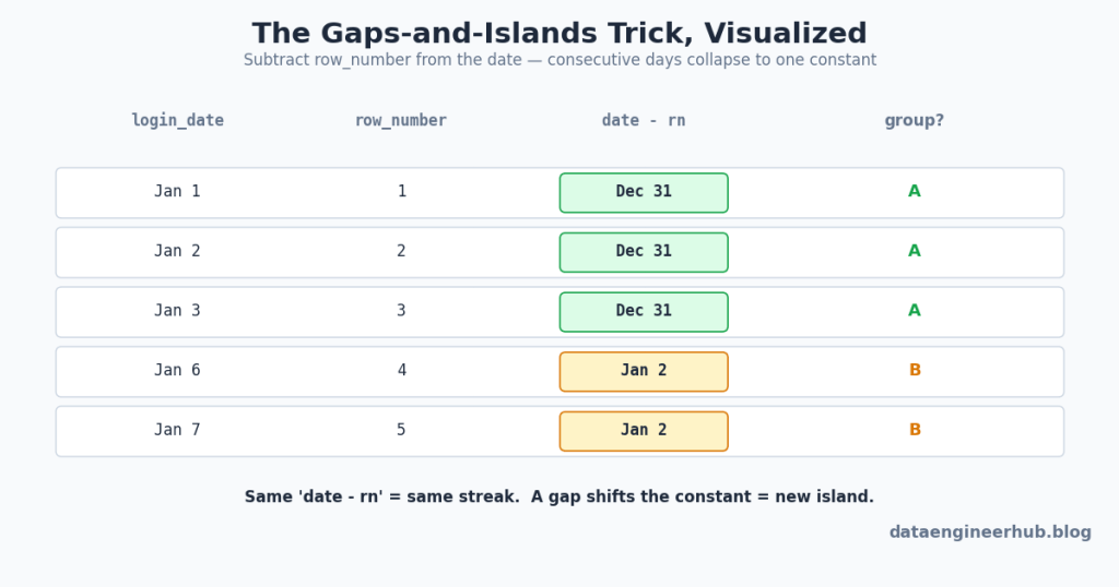
    Why it works: for consecutive days the row number grows in lockstep with the date, so date − rn is constant. The moment a day is skipped, the constant jumps — and that jump is your new streak boundary.

    WITH distinct_logins AS (
      SELECT DISTINCT user_id, login_date FROM logins
    ),
    numbered AS (
      SELECT user_id, login_date,
             ROW_NUMBER() OVER (PARTITION BY user_id ORDER BY login_date) AS rn
      FROM distinct_logins
    ),
    login_groups AS (
      SELECT user_id, login_date,
             DATE_SUB(login_date, INTERVAL rn DAY) AS grp
      FROM numbered
    )
    SELECT user_id,
           MIN(login_date) AS streak_start,
           MAX(login_date) AS streak_end,
           COUNT(*)        AS streak_length
    FROM login_groups
    GROUP BY user_id, grp
    HAVING COUNT(*) >= 5
    ORDER BY user_id;

    The follow-up: “what if you need to detect the gaps themselves, not the streaks?” Switch to LAG() — compare each row to the previous login, flag where the difference isn’t 1 day, and cumulative-sum those flags into group IDs. Same idea, different vehicle. Note the DISTINCT up front: duplicate logins on the same day would silently break the row-number arithmetic.

    2. Top-N per group

    Keywords: top 3 per department, highest/lowest per group, latest record, first/last. The single most common window-function question. Partition by the group, order by the metric, filter on the rank.

    WITH ranked AS (
      SELECT *,
             ROW_NUMBER() OVER (PARTITION BY department ORDER BY salary DESC) AS rn
      FROM employees
    )
    SELECT * FROM ranked WHERE rn <= 3;

    The follow-up you must nail: “what if two people tie on salary?” That’s the interviewer probing whether you know the three ranking functions — and this is one of the most common trip-ups, so know it cold: ROW_NUMBER() gives 1,2,3 with an arbitrary tiebreaker; RANK() gives 1,1,3 (ties share a rank, next rank skips); DENSE_RANK() gives 1,1,2 (ties share, no gap). If the question is “top 3 salaries” and ties should all count, you want DENSE_RANK(), not ROW_NUMBER(). For the “latest record per user” variant, it’s the identical shape with ORDER BY created_at DESC and WHERE rn = 1.

    3. Running totals / cumulative metrics

    Keywords: running total, cumulative, so far, progressive. The frame does the work: SUM(x) OVER (ORDER BY dt ROWS BETWEEN UNBOUNDED PRECEDING AND CURRENT ROW).

    WITH daily_revenue AS (
      SELECT DATE(created_at) AS order_date, SUM(amount) AS revenue
      FROM orders
      GROUP BY DATE(created_at)
    )
    SELECT order_date,
           SUM(revenue) OVER (
             ORDER BY order_date
             ROWS BETWEEN UNBOUNDED PRECEDING AND CURRENT ROW
           ) AS running_total
    FROM daily_revenue;

    The follow-up: “now show each user’s running total and the global running total in the same query.” That tests whether you understand that two window functions can carry different PARTITION BY clauses side by side — a per-user frame partitioned by user_id, and a global frame with no partition — which usually means aggregating to user-day and day grains first, then combining.

    4. Event → state transformation

    Keywords: headcount over time, active subscriptions per day, “build the metric then track it.” Here the metric doesn’t exist in the data — you construct it from events. The classic is daily headcount: turn each hire into +1 and each termination into −1, then take a running sum over a date spine.

    WITH RECURSIVE date_spine AS (
        SELECT MIN(hire_date) AS dt FROM employee
        UNION ALL
        SELECT DATE_ADD(dt, INTERVAL 1 DAY) FROM date_spine
        WHERE dt < CURRENT_DATE()
    ),
    changes AS (
        SELECT hire_date AS dt, +1 AS delta FROM employee
        UNION ALL
        SELECT termination_date AS dt, -1 AS delta
        FROM employee WHERE termination_date IS NOT NULL
    ),
    daily_change AS (
        SELECT dt, SUM(delta) AS tdelta FROM changes GROUP BY dt
    )
    SELECT d.dt,
           SUM(COALESCE(c.tdelta, 0)) OVER (
             ORDER BY d.dt ROWS BETWEEN UNBOUNDED PRECEDING AND CURRENT ROW
           ) AS headcount
    FROM date_spine d
    LEFT JOIN daily_change c ON d.dt = c.dt
    ORDER BY d.dt;

    The “+1/−1 delta then running sum” trick generalizes to any state-from-events problem: concurrent sessions, active subscriptions, inventory on hand.

    5. Rolling / moving windows

    Keywords: 7-day moving average, 30-day active users, trailing metric. Same window machinery as running totals, but a bounded frame. The gotcha that separates candidates: ROWS BETWEEN 6 PRECEDING AND CURRENT ROW is 7 rows, not 6.

    SELECT sale_date, daily_sales,
           AVG(daily_sales) OVER (
             ORDER BY sale_date
             ROWS BETWEEN 6 PRECEDING AND CURRENT ROW
           ) AS moving_avg_7d
    FROM daily_sales;

    Window frames are worth truly internalizing, because half these patterns are just different frame boundaries over the same OVER() skeleton:

    Every rolling metric is just a choice of frame boundaries relative to the current row. And the ROWS-vs-RANGE distinction at the bottom is a favorite senior-level probe — worth knowing why one is deterministic.

    The ROWS-vs-RANGE trap: the default frame for SUM() OVER (ORDER BY dt) is actually RANGE, which groups all rows sharing the same ORDER BY value into one step — so two orders on the same date both get the day-end total, not their individual accumulation. ROWS treats each physical row independently. For running totals and time series, prefer ROWS to avoid unintended grouping on ties; being able to explain that difference unprompted signals real depth.

    6. Cohort / retention analysis

    Keywords: retention, cohort, week 0 / week 1, signup behavior. Ubiquitous at product companies. The shape is always: assign each user a cohort (their first-activity period), then measure activity by offset from that cohort.

    WITH user_cohort AS (
      SELECT user_id, DATE_TRUNC('week', MIN(activity_date)) AS cohort_week
      FROM user_activity GROUP BY user_id
    ),
    user_activities AS (
      SELECT a.user_id, c.cohort_week,
             DATE_TRUNC('week', a.activity_date) AS activity_week
      FROM user_activity a
      JOIN user_cohort c ON a.user_id = c.user_id
    ),
    cohort_size AS (
      SELECT cohort_week, COUNT(DISTINCT user_id) AS total_users
      FROM user_cohort GROUP BY cohort_week
    )
    SELECT ua.cohort_week,
           DATEDIFF('week', ua.cohort_week, ua.activity_week) AS weeks_since_signup,
           COUNT(DISTINCT ua.user_id) AS active_users,
           COUNT(DISTINCT ua.user_id) * 1.0 / cs.total_users AS retention_rate
    FROM user_activities ua
    JOIN cohort_size cs ON ua.cohort_week = cs.cohort_week
    GROUP BY ua.cohort_week, weeks_since_signup, cs.total_users
    ORDER BY ua.cohort_week, weeks_since_signup;

    The three-CTE structure — cohort assignment, activity-with-offset, cohort size for the denominator — is the reusable skeleton. Retention rate is just active-at-offset divided by the week-0 size.

    7. Self-join logic

    Keywords: compared to previous, more than their manager, bought A but not B. Any time you compare rows within the same table. The “A but not B” version is a clean anti-join:

    SELECT DISTINCT a.user_id
    FROM purchases a
    LEFT JOIN purchases b
      ON a.user_id = b.user_id AND b.product = 'B'
    WHERE a.product = 'A' AND b.user_id IS NULL;

    The trap here is NULLs. The instinct is often WHERE user_id NOT IN (SELECT user_id FROM purchases WHERE product='B') — but if that subquery returns even one NULL, NOT IN yields zero rows, silently. The LEFT JOIN ... IS NULL anti-join above is immune. Many “compare to previous row” self-joins are also better expressed with LAG(), which is cheaper than a correlated subquery and reads more clearly.

    8. Time-series expansion (date spine)

    Keywords: daily trend, fill missing dates, continuous timeline, “even days with zero.” The fix for gaps in a report is to generate the complete calendar and LEFT JOIN your data onto it, so missing periods become explicit zeros instead of vanishing rows.

    WITH RECURSIVE months AS (
        SELECT DATE_FORMAT(MIN(hire_date), '%Y-%m-01') AS month_start FROM employees
        UNION ALL
        SELECT DATE_ADD(month_start, INTERVAL 1 MONTH) FROM months
        WHERE month_start < DATE_FORMAT(CURRENT_DATE(), '%Y-%m-01')
    )
    SELECT m.month_start, COALESCE(SUM(x.metric), 0) AS metric
    FROM months m
    LEFT JOIN some_table x ON DATE_FORMAT(x.dt, '%Y-%m-01') = m.month_start
    GROUP BY m.month_start
    ORDER BY m.month_start;

    The production aside worth saying out loud: recursive date spines that recompute headcount by rescanning all employees every month are fine in an interview but expensive at scale. Mentioning that you’d back this with a precomputed monthly_headcount snapshot table in production — built by an incremental pipeline rather than recomputed each run — is exactly the kind of comment that separates a senior candidate, and it ties directly to not reprocessing what didn’t change.

    9. Percentiles / distribution

    Keywords: top 10%, percentile, ranking distribution. This is where NTILE()PERCENT_RANK(), and DENSE_RANK() live. “Top 10% of employees by rating” has a naive form and a fair form, and the interviewer usually wants the fair one:

    -- Fair version: handles ties at the cutoff correctly
    WITH latest_rating AS (
      SELECT emp_id, rating,
             ROW_NUMBER() OVER (PARTITION BY emp_id ORDER BY review_date DESC) AS rnk
      FROM performance_reviews
    ),
    ranked AS (
      SELECT *,
             DENSE_RANK() OVER (ORDER BY rating DESC) AS bucket,
             COUNT(*)     OVER () AS total_count
      FROM latest_rating WHERE rnk = 1
    )
    SELECT * FROM ranked WHERE bucket <= CEIL(0.10 * total_count);

    NTILE(10) forces exactly ten equal-sized buckets (take bucket 1); the DENSE_RANK approach is fairer when many people share the boundary rating. The killer follow-up is point-in-time correctness: “employees change departments over time — attribute each rating to the department they were in then.” That forces a slowly-changing-dimension join on a date range (start_date <= review_date < end_date) instead of a naive join to the employee’s current department — and getting that right is a strong signal.

    10. Detect overlapping date ranges

    Keywords: booking conflicts, overlapping subscriptions, double-booked, schedule clash. The elegant move is to reason about when ranges don’t overlap, then invert. Two ranges miss each other only if one ends before the other starts:

    -- Non-overlap:  a.end < b.start  OR  b.end < a.start
    -- Invert (De Morgan) -> the standard overlap condition:
    SELECT s1.customer_id,
           s1.subscription_id AS sub_1,
           s2.subscription_id AS sub_2
    FROM subscriptions s1
    JOIN subscriptions s2
      ON s1.customer_id = s2.customer_id
     AND s1.subscription_id < s2.subscription_id   -- avoid self- and duplicate pairs
     AND s1.end_date >= s2.start_date
     AND s2.end_date >= s1.start_date;

    Two details interviewers check: the s1.id < s2.id condition (so you don’t compare a row to itself or count each pair twice), and that you derived the overlap condition rather than memorized it — walking through the two non-overlap cases and applying De Morgan’s law is the move that earns the nod.

    Putting it together: the combined question

    Real interviews often stack two or three patterns. “Monthly revenue for completed 2025 orders, with the change vs the previous month, showing all 12 months even when revenue is zero” is three patterns at once: conditional filtering, a date spine (all 12 months), and LAG() for the month-over-month delta — over a base that first aggregates order_items to order grain before summing to month grain. If you can see it as “aggregate → spine → LAG” instead of one intimidating blob, you’ve already won. The recognition reflex is the whole skill; the syntax is just spelling.

    The gotchas nobody warns you about

    NOT IN with a NULL returns nothing. One NULL in the subquery and NOT IN silently yields zero rows. Use NOT EXISTS or a LEFT JOIN ... IS NULL anti-join for exclusions, every time.

    ROWS ≠ RANGE, and the default is RANGE. SUM() OVER (ORDER BY dt) groups tied values into one step. For a true row-by-row running total, spell out ROWS BETWEEN UNBOUNDED PRECEDING AND CURRENT ROW.

    “6 PRECEDING” is a 7-row window. Off-by-one on frame bounds silently produces the wrong average. Count the current row.

    ROW_NUMBER vs RANK vs DENSE_RANK is a tie question in disguise. When the interviewer says “what if they tie,” they’re testing which one you’d swap to. Have the 1,2,3 / 1,1,3 / 1,1,2 distinction ready.

    Wrapping a date column in a function kills index/pruning use. Prefer hire_date >= DATE_SUB(CURRENT_DATE(), INTERVAL 6 MONTH) over TIMESTAMPDIFF(MONTH, hire_date, ...) <= 6 — same logic, but the range predicate can use metadata the function form throws away.

    The one principle

    You don’t pass a SQL interview by knowing more syntax — you pass it by recognizing that the strange-sounding question in front of you is one of about ten patterns you’ve already solved a dozen times. Learn the keyword that gives each pattern away, learn the one core trick behind it, and practice the recognition until it’s instant. Then the interview stops being a memory test and becomes what it should be: a conversation about the interesting variation, conducted in a language you already speak fluently.


    Related reading: Why senior engineers write SQL differently · Why SQL is still the most valuable skill · Don’t recompute what didn’t change · Making these queries fast in production

  • Why Senior Data Engineers Write SQL Differently (With Examples)

    Why Senior Data Engineers Write SQL Differently (With Examples)

    I once inherited a revenue report that had been green for fourteen months. Every morning it ran, populated a dashboard, and nobody questioned it. Then a new CFO asked why the data warehouse said Q2 regional revenue was $4.1M while the finance system said $1.3M. Same source data. The query had no error, no failed test, no warning. It had one join. Somewhere upstream, an orders table was joined to order_items, and a downstream SUM was quietly counting each order’s total once for every line item on it. A three-line-item order got counted three times. For fourteen months.

    The engineer who wrote it was competent. The SQL was readable. It followed every rule in the “write clean SQL” playbook — named columns, tidy formatting, sensible aliases. And it was still catastrophically wrong, because clean and correct are different things. That gap is what actually separates senior SQL from junior SQL, and it’s a deeper gap than the usual advice about CTEs and naming suggests. The readability stuff is real and I’ll get to it, but if that’s all you fix, you’ll write beautifully formatted queries that overstate revenue by 3x. Senior SQL is different along three axes at once — correctnesscost, and change-safety — and only the third is about how the code looks. This isn’t abstract, by the way: I’ve argued that SQL is the highest-leverage skill on a data team right now, and this is exactly why — the language is easy, the judgment is not.

    TL;DR

    • → A query that runs clean can still be wrong; the most expensive SQL bugs produce plausible numbers, not errors.
    • → Track the grain of every CTE — joining before you aggregate is the single most common cause of silently inflated totals.
    • → NOT IN (subquery) returns zero rows if the subquery contains a single NULL; seniors use NOT EXISTS for anti-joins.
    • → Deduping with QUALIFY ROW_NUMBER() and a tie-broken ORDER BY is reproducible; SELECT DISTINCT and untied ROW_NUMBER are not.
    • → Wrapping a filter column in a function (DATE(ts) = ...) and using SELECT * both defeat the engine’s ability to skip data, and that shows up on the bill.
    • → CTEs aren’t just prettier — each one is a debugging checkpoint you can query in isolation when a number looks wrong.
    • → Junior engineers optimize to make the query run; senior engineers optimize so the next change, and the next reader, don’t create a new bug.

    Senior SQL isn’t clever SQL

    There’s a myth that senior engineers write dense, impressive queries full of tricks. The opposite is true. The most senior SQL I’ve reviewed is almost boring to read — because the author spent their cleverness on being right and cheap, not on being concise. The comparison above captures the pattern: at every decision point there’s a lazy default that works on your laptop against 100 rows, and a deliberate choice that survives contact with production data. The rest of this article is the “why” behind the right-hand column, with real SQL for each.

    Correctness #1: the grain trap that triples your revenue

    This is the bug from the intro, and it’s worth seeing in code because it looks completely innocent. The business question: total spend per customer. There’s an orders table and an order_items table. Here’s the query that ran for fourteen months:

    -- WRONG: order_total is counted once per line item
    SELECT
        o.customer_id,
        SUM(o.order_total) AS total_spend
    FROM orders o
    JOIN order_items oi ON oi.order_id = o.order_id
    WHERE o.status <> 'refunded'
    GROUP BY o.customer_id;

    The join changes the grain. Before the join, orders has one row per order. After joining order_items, an order with three line items becomes three rows — each carrying the full order_total. The SUM then adds that total three times. Nothing errors; the number is just inflated by however many items the average order has.

    The join multiplied the rows; the SUM multiplied the money. The fix is to aggregate at the right grain before joining.

    The senior version aggregates order_items down to one row per order first, so every later step operates on a known grain:

    WITH order_revenue AS (              -- grain: one row per order
        SELECT
            oi.order_id,
            SUM(oi.quantity * oi.unit_price) AS order_total
        FROM order_items oi
        GROUP BY oi.order_id
    )
    SELECT
        o.customer_id,                   -- grain: one row per customer
        SUM(orv.order_total) AS total_spend
    FROM orders o
    JOIN order_revenue orv ON orv.order_id = o.order_id
    WHERE o.status <> 'refunded'
    GROUP BY o.customer_id;

    The habit that prevents this bug isn’t a syntax rule — it’s asking “what is the grain of this result?” after every join and every CTE. Seniors annotate it, as in the comments above. This is the same class of silent failure I wrote about in why passing dbt tests still ship bad data: uniqueness and not-null tests would both pass on the wrong query above, because the rows really are unique and non-null. They’re just counted too many times.

    Correctness #2: NOT IN will betray you

    You need a win-back list: customers with no orders in the last 90 days. The obvious query:

    -- WRONG if orders.customer_id contains any NULL
    SELECT customer_id, email
    FROM customers
    WHERE customer_id NOT IN (
        SELECT customer_id
        FROM orders
        WHERE order_date >= CURRENT_DATE - 90
    );

    If a single row in that subquery has a NULL customer_id — a guest checkout, a bad load, a soft-deleted account — this query returns zero rows. Not an error. An empty result that looks like “nobody qualifies.” The reason is SQL’s three-valued logic: NOT IN is defined as “not equal to any,” and comparing anything to NULL yields UNKNOWN, which poisons the whole condition so no row is ever selected. This is spec-mandated behavior, documented in PostgreSQL’s logical operators reference, and it behaves the same across every compliant engine.

    The senior default is an anti-join with NOT EXISTS, which is immune to the NULL problem because it tests row existence, not value equality:

    SELECT c.customer_id, c.email
    FROM customers c
    WHERE NOT EXISTS (
        SELECT 1
        FROM orders o
        WHERE o.customer_id = c.customer_id
          AND o.order_date >= CURRENT_DATE - 90
    );

    Rule of thumb worth internalizing: reach for NOT EXISTS over NOT IN every time a subquery is involved, unless you have proven the column is non-nullable. It’s not a style preference; it’s a correctness guarantee.

    Correctness #3: dedup that returns the same rows twice

    Deduplication is where juniors reach for SELECT DISTINCT and seniors reach for a window function — and the difference is about determinism, not taste. Say raw_orders has duplicate order_ids from an at-least-once ingestion, and you want the latest version of each. DISTINCT can’t express “latest”; it just collapses fully identical rows. And ROW_NUMBER without a tie-break silently picks an arbitrary row when the sort column ties — so the same pipeline can emit different rows on different runs, which is a nightmare to debug.

    The senior pattern uses QUALIFY to filter on a window function inline, with a deterministic ordering:

    SELECT order_id, customer_id, status, order_total, updated_at
    FROM raw_orders
    QUALIFY ROW_NUMBER() OVER (
        PARTITION BY order_id
        ORDER BY updated_at DESC, ingested_at DESC   -- tie-break = determinism
    ) = 1;
    +----------+-------------+----------+-------------+---------------------+
    | order_id | customer_id | status   | order_total | updated_at          |
    +----------+-------------+----------+-------------+---------------------+
    |      101 |        4471 | shipped  |      150.00 | 2026-07-20 14:02:11 |
    |      102 |        2210 | placed   |      200.00 | 2026-07-21 09:15:40 |
    |      103 |        8890 | returned |      250.00 | 2026-07-21 18:44:02 |
    +----------+-------------+----------+-------------+---------------------+

    The second column in the ORDER BY is the tell. A junior stops at updated_at DESC; a senior adds a unique tie-breaker so that when two rows share an updated_at, the query still picks the same one every single run. Reproducibility is a correctness property, and non-deterministic SQL is a close cousin of the “same input, different output” problem — except here you can actually eliminate it.

    Cost: write SQL the engine is allowed to skip

    Correctness keeps you employed; cost keeps you promoted. On columnar cloud warehouses, two junior habits quietly multiply what a query scans. Consider:

    -- Scans every column, every micro-partition
    SELECT *
    FROM events
    WHERE DATE(event_ts) = '2026-07-01';

    Two problems. SELECT * forces the engine to read every column, including fat JSON and audit fields nobody asked for. And wrapping event_ts in DATE() means the optimizer can’t use the raw timestamp to prune partitions — it has to compute a function over every row first. The senior rewrite selects only what it needs and expresses the filter as a half-open range on the bare column, which lets the engine skip whole partitions it knows can’t match:

    SELECT event_id, user_id, event_type
    FROM events
    WHERE event_ts >= '2026-07-01'
      AND event_ts <  '2026-07-02';

    If you want the mechanics of why this works — how pruning and partition elimination actually happen — I walked through it in what really happens when you run a query in Snowflake, and why re-running the same query can be nearly free in how the warehouse cache actually works.

    The cost math

    Put rough numbers on it. Say events is 2 TB across 40 columns, roughly evenly sized, holding one year of data. The junior query scans close to the full 2 TB. Selecting only the three columns you need cuts that to about 150 GB (three of forty columns). Adding the prunable date range drops it to one day out of ~365 — on the order of 400 MB actually read. That’s a ~5,000x reduction in bytes scanned, on a warehouse you’re billed for by the second, from two changes that took ten seconds to make. This is the same discipline behind not rebuilding models that didn’t change, which is the whole premise of dbt state-based selection — and it’s why teams serious about spend even push analytics to cheaper engines like DuckDB for dev workloads.

    Change-safety: CTEs as checkpoints, not decoration

    This is the axis the “clean SQL” advice usually covers, and it’s genuinely important — just not sufficient on its own. Structuring a query as a sequence of named CTEs (recent_orders → order_revenue → customer_summary) does more than read nicely. Each CTE is a checkpoint you can inspect in isolation: when a customer is missing from the output, you don’t mentally execute a nested monster, you run SELECT * FROM order_revenue WHERE order_id = 8821 and walk the stages until the row disappears. That’s the difference between a five-minute debug and a fifty-minute one.

    The other half of change-safety is treating your SELECT list as a contract. SELECT * in a model means that the day someone adds a gdpr_deletion_requested column upstream, it silently flows into every downstream dashboard — the exact class of break I covered in how one renamed column kills a pipeline. An explicit column list is a promise about what this query returns, and promises are what let the next engineer change things without fear. If you want this enforced at the project level rather than per query, the layering conventions in structuring dbt projects in Snowflake are the natural home for it.

    The gotchas nobody warns you about

    DISTINCT is often a fan-out cover-up. If you added SELECT DISTINCT to “fix” duplicate rows, you probably have a grain bug upstream and are papering over it. DISTINCT hides the symptom and keeps the doubled aggregates.

    BETWEEN on timestamps is a silent off-by-one. event_ts BETWEEN '2026-07-01' AND '2026-07-02' includes midnight of the second day, double-counting boundary rows. Half-open ranges (>= and <) are the senior default for exactly this reason.

    COUNT(column) and COUNT(*) are not the same. COUNT(col) skips NULLs; COUNT(*) counts rows. Using the wrong one turns a data-quality problem into a wrong metric that looks fine.

    RANK and ROW_NUMBER dedup differently. RANK() assigns ties the same number, so QUALIFY RANK() = 1 can keep multiple rows per key. For “exactly one row per key,” it must be ROW_NUMBER().

    ORDER BY inside a CTE or view is not guaranteed to hold. The engine is free to reorder unless the outermost query sorts. If order matters downstream, sort where the data is consumed, not where it’s defined.

    The one principle

    Junior engineers write SQL that returns the right answer today; senior engineers write SQL that can’t quietly start returning the wrong one. The clean formatting, the CTEs, the explicit columns — those are the visible surface. Underneath is a habit of assuming your data is messier than the demo, your query will be re-run on data you haven’t seen, and the next person to touch it won’t know what you knew. Write for that world, and “senior SQL” stops being a style and becomes a form of insurance.


    Related reading: Why passing dbt tests still ship bad data · What really happens when you run a query · How one renamed column kills a pipeline · Why SQL is the most valuable skill in AI · Snowflake QUALIFY reference · PostgreSQL three-valued logic

  • 5 Real-World SQL Portfolio Projects That Actually Get You Hired

    5 Real-World SQL Portfolio Projects That Actually Get You Hired

    A hiring manager I know keeps a folder of rejected portfolio links. Not to be cruel — to remember the pattern. Out of roughly forty SQL “projects” she reviewed for one analytics-engineer opening, thirty-one were the same customer-churn notebook off the same Kaggle CSV, with the same three queries, ending on the same bar chart. She stopped opening them after about the fifteenth. The one candidate she did call had used the identical dataset as everyone else — but she’d written a paragraph explaining that 4,200 rows had a tenure of zero and a churn flag of one, which is impossible, and how she decided to handle them. That paragraph got her the interview. The SQL didn’t.

    That is the thing nobody tells you when you start building a data portfolio: the query is table stakes. Everyone can write a GROUP BY. What almost nobody does is show that they can think about data the way it actually behaves in production — dirty, contradictory, and full of rows that break your assumptions. If you’re weighing whether SQL is even worth the investment in an AI-saturated market, it still is; I’ve argued at length about why SQL quietly became the most valuable skill in the modern stack. This article is the follow-on: five projects genuinely worth building, the public repositories and datasets to build them from, and — the part that matters — what to add to each so it doesn’t land in the rejected folder.

    TL;DR

    • → Hiring managers reject SQL portfolios for sameness, not syntax errors; the differentiator is documented judgment about messy data, not a cleaner JOIN.
    • → Five projects cover the skills employers actually screen for: churn analysis, a Bronze/Silver/Gold data warehouse, sales analysis, customer segmentation, and healthcare KPIs.
    • → A Bronze/Silver/Gold data-warehouse build is the single highest-signal SQL portfolio project because it proves modeling and ETL thinking, not just querying.
    • → Window functions (NTILERANKROW_NUMBER) separate a beginner portfolio from a mid-level one faster than any other SQL feature.
    • → Use real, messy public data — NYC TLC trip records, open GitHub project datasets — instead of the pre-cleaned Kaggle CSV everyone else submitted.
    • → Every project needs a written “what I found and what I’d do about it” section; a small, well-explained project beats a large one with no story.
    • → You can run all five locally for free with DuckDB or SQLite — no cloud warehouse and no credit-card required.

    Why most SQL portfolios get skipped in 30 seconds

    Reviewers don’t read portfolios top to bottom. They scan for a reason to say no, because they have forty of them and one afternoon. A wall of SELECT statements with no narrative gives them that reason instantly. So does a project that’s obviously a tutorial you followed step-for-step, because a tutorial proves you can type, not that you can decide.

    The uncomfortable truth is that clean, green output is not evidence of good work. I’ve written before about how tests can pass while you’re still shipping bad data, and the same trap applies to portfolios: a query that runs without error can still be answering the wrong question on data you never inspected. A reviewer who has been burned by exactly that in production is looking for the opposite signal — someone who checked.

    This is also why I’m lukewarm on stacking certifications as a substitute for building things; I’ve made the full case for why a certificate rarely moves a hiring decision. A project where you can point at a specific decision you made — “I bucketed tenure this way because the raw values were bimodal” — does the thing a certificate can’t. It shows judgment.

    So as you read the five projects below, treat the query as the easy 20%. The 80% that gets you hired is the layer on top: the data-quality checks, the edge cases you caught, and the plain-English conclusion.

    The five projects worth building

    These five map to the roles most people are actually applying for — analyst, analytics engineer, BI developer — and between them they exercise every SQL skill a screener looks for. For each one I’ve noted a real public repository or dataset to start from, and the one addition that lifts it above the crowd.

    1. E-commerce customer churn analysis

    Churn is the most common portfolio project for a reason: it’s a real business problem with a clear money consequence, and it maps cleanly to SQL. You take a table of customers with attributes like tenure, complaint counts, satisfaction scores, order frequency, coupon usage, and days since last order, and you find the patterns that predict who leaves. A good public starting point is the open-source Ecommerce Customer Churn Analysis repository, which ships the raw CSV and a full query file you can read, critique, and improve rather than copy.

    The skills on display are aggregation, conditional logic, and segmentation. Here’s the kind of query that belongs in this project — churn rate bucketed by tenure, which immediately tells a retention story:

    SELECT
        tenure_bucket,
        COUNT(*)                                  AS customers,
        SUM(churned)                              AS churned_customers,
        ROUND(100.0 * SUM(churned) / COUNT(*), 1) AS churn_rate_pct
    FROM (
        SELECT
            customer_id,
            CASE WHEN churn = 1 THEN 1 ELSE 0 END AS churned,
            CASE
                WHEN tenure < 6  THEN '0-5 months'
                WHEN tenure < 12 THEN '6-11 months'
                WHEN tenure < 24 THEN '12-23 months'
                ELSE '24+ months'
            END AS tenure_bucket
        FROM ecommerce_churn
    ) t
    GROUP BY tenure_bucket
    ORDER BY churn_rate_pct DESC;
    Run it and you get something like this:
    
    +---------------+-----------+-------------------+----------------+
    | tenure_bucket | customers | churned_customers | churn_rate_pct |
    +---------------+-----------+-------------------+----------------+
    | 0-5 months    |      1846 |               912 |           49.4 |
    | 6-11 months   |      1204 |               331 |           27.5 |
    | 12-23 months  |      1098 |               142 |           12.9 |
    | 24+ months    |       503 |                28 |            5.6 |
    +---------------+-----------+-------------------+----------------+

    What to add that nobody else does: before you compute a single rate, profile the data and write down what’s wrong with it. Customers with a tenure of zero but a churn flag set. Satisfaction scores outside the documented range. Duplicate customer IDs. Then state your handling decision and why. That paragraph is the reason a reviewer keeps reading.

    2. A Bronze/Silver/Gold data warehouse

    If you build only one project from this list, build this one. It’s the highest-signal thing on the page because it proves you understand how real data systems are assembled — ingestion, cleansing, and modeling into fact and dimension tables — not just how to query a table someone else prepared. The SQL Data Warehouse Project by Data With Baraa is the gold-standard reference here: it’s MIT-licensed, has hundreds of forks, and walks the full Medallion (Bronze → Silver → Gold) architecture using ERP and CRM CSV sources loaded into a SQL database, then modeled into a star schema.

    You’ll practice ETL sequencing, data cleaning, and dimensional modeling. If you want to understand the modeling layer more deeply — where the real design decisions live — my guide on structuring a warehouse project into staging, intermediate, and mart layers maps almost one-to-one onto Bronze/Silver/Gold, and it’ll help you explain why your layers are split the way they are.

    What to add that nobody else does: a data catalog and naming conventions. Two short Markdown files — one documenting every column in your Gold tables, one stating your table/column naming rules — signal “I’ve worked on a team” louder than any query. It’s also the thing that separates a warehouse project from a pile of scripts.

    3. Sales data analysis

    Sales analysis connects SQL directly to business performance, which makes it the easiest project to narrate to a non-technical interviewer. You answer questions a real stakeholder asks: which products drive revenue, how revenue trends month over month, which customer cohorts spend the most, whether there’s seasonality. The skills are joins, date functions, sorting, filtering, and time-based grouping.

    This is a great one to build on genuinely large, genuinely messy public data instead of a tidy sample. The NYC Taxi & Limousine Commission trip records are a government-published dataset running to millions of rows per month, with real quirks — negative fares, zero-distance trips, timestamps out of order. Treating trips as “sales” and analyzing revenue by hour, zone, and payment type gives you a portfolio piece at a scale most candidates never touch. And you don’t need a cluster to do it: I’ve made the case for why you should stop spinning up Spark for datasets this size — DuckDB will chew through a month of trip data on your laptop.

    What to add that nobody else does: a “so what” for every chart. Don’t just show that December revenue is up. Say what a business would do about it. The analysis is the input; the recommendation is the deliverable.

    4. Bank customer segmentation

    Segmentation is where you graduate from beginner SQL to mid-level SQL, because it’s the natural home for window functions. You take a banking-style dataset of customers, transactions, and regions, and you rank customers by value, flag dormant versus active accounts, and score regional performance. Employers in fintech and financial analytics screen hard for CTEsNTILERANK, and PARTITION BY — and this project shows all of them at once.

    WITH customer_value AS (
        SELECT
            customer_id,
            region,
            SUM(transaction_amount) AS total_spend,
            COUNT(*)                AS txn_count,
            MAX(transaction_date)   AS last_txn
        FROM bank_transactions
        GROUP BY customer_id, region
    )
    SELECT
        customer_id,
        region,
        total_spend,
        NTILE(4) OVER (ORDER BY total_spend DESC)  AS value_quartile,
        RANK()   OVER (PARTITION BY region
                       ORDER BY total_spend DESC)  AS rank_in_region
    FROM customer_value
    ORDER BY total_spend DESC
    LIMIT 5;
    +-------------+---------+-------------+----------------+----------------+
    | customer_id | region  | total_spend | value_quartile | rank_in_region |
    +-------------+---------+-------------+----------------+----------------+
    |       10427 | South   |    284119.50 |              1 |              1 |
    |       10088 | West    |    271004.20 |              1 |              1 |
    |       10391 | South   |    259847.75 |              1 |              2 |
    |       10142 | North   |    244310.00 |              1 |              1 |
    |       10265 | West    |    238900.10 |              1 |              2 |
    +-------------+---------+-------------+----------------+----------------+

    What to add that nobody else does: define your segments before you write the SQL, in business terms, and defend the thresholds. “High-value” meaning top quartile by spend is a choice; so is defining “dormant” as no transaction in 90 days. Writing down why you drew the lines where you did is the difference between analysis and arbitrary bucketing.

    5. Healthcare data analysis

    Healthcare rounds out the set because it proves you can work with domain-specific, meaningful data: patient records, conditions, hospitals, insurance providers, admission types, and billing. You explore which conditions are most common, how billing varies by condition, which hospitals see the most volume, and how admission types differ across patient groups. The SQL skills — grouping, filtering, joins, aggregates — overlap with sales analysis, but the domain framing shows range.

    What to add that nobody else does: a KPI rollup with definitions. Healthcare reviewers care about correctness of metrics. Publishing a small set of KPIs (average length of stay, cost per admission type, readmission proxy) with an explicit definition for each shows you understand that a metric is only as good as its definition — the same discipline that keeps a real reporting layer trustworthy.

    Where to get data that isn’t the same tired CSV

    The fastest way to blend into the rejected folder is to use the exact pre-cleaned dataset every tutorial uses. Three better sources: open GitHub project repositories that ship their own raw CSVs (like the two linked above), government open-data portals such as the NYC TLC records for genuine scale and mess, and Kaggle for breadth when you want a specific domain. The rule of thumb: the messier and more real the source, the more your data-quality work has something to actually do — which is the whole point.

    You do not need cloud infrastructure for any of this. All five projects run locally on DuckDB or SQLite for free, and if you later want to show you can operate against a warehouse without burning money, my walkthrough on querying warehouse data through DuckDB to cut costs covers the hybrid pattern. For the ingestion side of the warehouse project, a small Python loading script turns “I loaded CSVs” into “I built a repeatable pipeline.”

    How to actually spend your time

    Most people invert the effort. They spend 80% of their time writing more queries and 20% on everything else, then wonder why the portfolio reads like homework. Flip it. A realistic budget for one strong project looks closer to this: roughly 15% profiling and cleaning the data, 25% writing the core SQL, 20% catching and documenting edge cases, and 40% on the write-up — the README, the data-quality notes, and the plain-English conclusions. The queries are the cheapest part to produce and the least differentiating. The narrative is expensive, rare, and exactly what gets remembered.

    This is also why one finished, deeply documented project beats five half-built ones. Depth is legible to a reviewer in a way that breadth isn’t. Five shallow churn notebooks read as one shallow churn notebook copied five times.

    The gotchas nobody warns you about

    A green query is not a correct query. The most dangerous portfolio bug is a query that runs, returns plausible numbers, and is silently wrong because you joined on a column with duplicates and fanned out your row counts. Always sanity-check totals before and after a join.

    Averages lie on skewed data, and money is always skewed. “Average transaction value” across a banking dataset is nearly meaningless when a handful of whales dominate. Reach for medians and percentiles, and mention explicitly why you did — it signals statistical maturity.

    Date handling is where portfolios quietly break. Time zones, mixed formats, and out-of-order timestamps in real datasets like the TLC records will wreck a naive monthly rollup. The candidate who noticed 200 trips with a drop-off before the pick-up looks far stronger than the one whose numbers were merely clean.

    Schema assumptions rot the moment upstream data changes. If a column you depend on gets renamed or retyped, your whole analysis silently produces garbage — the exact failure mode I unpack in the piece on how a single renamed column kills a pipeline. Documenting the schema you built against is cheap insurance and a strong signal.

    A dashboard is not a conclusion. Ending on a chart with no written interpretation is the most common way strong SQL gets wasted. The reviewer wants your read of the numbers, not a second job interpreting them.

    The one principle

    Your SQL proves you can query; your write-up proves you can think — and only one of those gets you hired. Pick one project from this list, use genuinely messy public data, and spend more time explaining your decisions than writing your queries. A small project with a documented point of view will beat a sprawling one with clean output and nothing to say, every single time.


    Related reading: Why SQL is the most valuable skill in AI (2026) · The problem with data engineering certifications · Structuring a warehouse project properly · Run it locally with DuckDB, not Spark · SQL Data Warehouse Project (GitHub) · NYC TLC trip record data

  • Building a Bulletproof ETL Audit Logger: Capturing Airflow Execution Context in Snowflake

    Building a Bulletproof ETL Audit Logger: Capturing Airflow Execution Context in Snowflake

    The 2 a.m. page said the pipeline “succeeded.” The dashboard was green. And the finance team was still staring at yesterday’s numbers, because one task in a forty-task DAG had quietly processed the wrong micro-batch window and nobody could prove when, or why, without SSH-ing into a worker and grepping logs by hand. That’s the gap between “DAG success/failure notifications” and actual observability: a green checkmark tells you the code didn’t throw, not that the right data moved in the right window at the right time.

    The fix isn’t a fancier alerting tool. It’s an audit table — a row written to Snowflake at the start and end of every single task, carrying the execution context Airflow already knows: which logical date this run is for, which try number, when the task actually started and finished, how long it took, and what it touched. Once that table exists, “when did this break and why is it slow” stops being an archaeology project and becomes a SELECT. This is the complete build: the Snowflake schema, the Airflow callback code that captures context at both ends of every task, and what the whole thing looks like when it runs.

    TL;DR

    → DAG-level success/failure is too coarse. Capture context at task start and task end for granular observability — timing, retries, and the exact micro-batch window per task.

    → Airflow exposes the execution context through callbacks: on_execute_callback fires right before a task runs (your “start” hook), and on_success_callback / on_failure_callback fire at the end. Each receives the full context dictionary.

    → The context carries what you need: logical_date (the micro-batch window), dag_run.run_idti.try_numberti.start_date, plus ds/ds_nodash for partition keys. In Airflow 3, access it programmatically with get_current_context() from the Task SDK.

    → Attach the callbacks once via default_args and every task in the DAG is audited automatically — no per-task boilerplate.

    → Ship rows to a centralized Snowflake PIPELINE_AUDIT_LOG table keyed by dag_id + task_id + run_id + try_number, with a START row and an END row per attempt so duration and status fall out of a simple query.

    → Once the data lands, debugging execution delays is a SELECT … ORDER BY duration_seconds DESC, and finding the slowest task in the slowest run is a window function, not a log grep.

    Why DAG-level notifications aren’t observability

    Diagram comparing “DAG success/failure” with “Per-task-attempt audit” using checklists. DAG shows overall result; audit tracks details like duration per task, attempts, logical date window, and slowest tasks.

    A DAG success signal answers one coarse question. The unit of observability you actually want is the task attempt.

    A DAG success notification answers one question: did the whole thing finish without an unhandled exception? That’s necessary and nowhere near sufficient. It can’t tell you which task in the chain was slow, whether a task silently ran on its second retry, which logical date window each task actually processed, or how today’s run compares to last week’s for the same task. Those are the questions you actually have during an incident, and log-grepping to answer them is how a five-minute diagnosis becomes a two-hour one.

    The unit of observability you want is the task attempt, not the DAG run. Every task attempt has a start, an end, a try number, and a logical date. If you record those four things for every attempt in one queryable place, you can answer “when did this get slow,” “which task is the bottleneck,” and “did this run process the window it should have” directly — and you can do it after the fact, without the worker still being alive.

    Step 1: the Snowflake audit table

    Start with the destination. The schema is deliberately simple — one row per task-attempt per phase (START and END), keyed so you can pair them up and compute duration. Keeping START and END as separate rows (rather than updating one row) means a task that dies hard still leaves its START row behind, which is itself a signal.

    CREATE TABLE IF NOT EXISTS ops.pipeline_audit_log (
        audit_id        STRING DEFAULT UUID_STRING(),
        dag_id          STRING       NOT NULL,
        task_id         STRING       NOT NULL,
        run_id          STRING       NOT NULL,
        try_number      NUMBER       NOT NULL,
        phase           STRING       NOT NULL,   -- 'START' | 'END'
        status          STRING,                  -- 'RUNNING' | 'SUCCESS' | 'FAILED'
        logical_date    TIMESTAMP_NTZ,           -- the micro-batch window
        event_time      TIMESTAMP_LTZ DEFAULT CURRENT_TIMESTAMP(),
        duration_sec    NUMBER,                  -- populated on END
        operator        STRING,
        map_index       NUMBER,                  -- for dynamically mapped tasks
        hostname        STRING,
        error_message   STRING,
        loaded_at       TIMESTAMP_LTZ DEFAULT CURRENT_TIMESTAMP()
    );

    A few deliberate choices. logical_date is stored as its own column because it’s the micro-batch window the task is for — distinct from event_time, the wall-clock moment the row was written. Conflating those two is the single most common audit-table mistake, and it’s exactly the confusion that hid the “wrong window” bug in the opening story. try_number is in the key because retries are first-class events you want to see, not noise to collapse. And map_index is there so dynamically mapped tasks (the .expand() fan-out) each get their own audit trail instead of blurring together.

    Step 2: extracting the execution context

    Airflow hands you everything through the context dictionary. The pieces that matter for auditing:

    def extract_audit_fields(context: dict) -> dict:
        """Pull the audit-relevant fields out of the Airflow context."""
        ti = context["ti"]                     # the TaskInstance
        dag_run = context["dag_run"]
    
        return {
            "dag_id":       ti.dag_id,
            "task_id":      ti.task_id,
            "run_id":       dag_run.run_id,
            "try_number":   ti.try_number,
            # logical_date is the micro-batch window this run is FOR.
            # Asset-triggered DAGs in Airflow 3 have none — fall back to None.
            "logical_date": context.get("logical_date"),
            "operator":     ti.operator,
            "map_index":    ti.map_index,
            "hostname":     ti.hostname,
            "start_date":   ti.start_date,
        }

    The distinction that trips people up: logical_date (formerly execution_date) is the window the run represents, which may be hours or months before the wall clock if you’re backfilling. ti.start_date is when the task actually began executing. You want both — one to know what the task processed, the other to know when and how long. In Airflow 3, if you’re inside task code rather than a callback, you get the same dictionary with from airflow.sdk import get_current_context and context = get_current_context().

    Step 3: the callbacks that fire at start and end

    This is the heart of it. on_execute_callback runs immediately before the task’s own code — that’s your START row. on_success_callback and on_failure_callback run after — those are your END rows, one carrying SUCCESS, the other FAILED plus the exception.

    from datetime import datetime, timezone
    
    def _write_audit_row(fields: dict) -> None:
        """Insert a single audit row into Snowflake via a reusable hook."""
        from airflow.providers.snowflake.hooks.snowflake import SnowflakeHook
        hook = SnowflakeHook(snowflake_conn_id="snowflake_ops")
        hook.run(
            """
            INSERT INTO ops.pipeline_audit_log
                (dag_id, task_id, run_id, try_number, phase, status,
                 logical_date, duration_sec, operator, map_index,
                 hostname, error_message)
            VALUES
                (%(dag_id)s, %(task_id)s, %(run_id)s, %(try_number)s,
                 %(phase)s, %(status)s, %(logical_date)s, %(duration_sec)s,
                 %(operator)s, %(map_index)s, %(hostname)s, %(error_message)s)
            """,
            parameters=fields,
        )
    
    def audit_on_start(context: dict) -> None:
        f = extract_audit_fields(context)
        f.update(phase="START", status="RUNNING",
                 duration_sec=None, error_message=None)
        _write_audit_row(f)
    
    def audit_on_success(context: dict) -> None:
        f = extract_audit_fields(context)
        duration = (datetime.now(timezone.utc) - f["start_date"]).total_seconds()
        f.update(phase="END", status="SUCCESS",
                 duration_sec=round(duration, 2), error_message=None)
        _write_audit_row(f)
    
    def audit_on_failure(context: dict) -> None:
        f = extract_audit_fields(context)
        duration = (datetime.now(timezone.utc) - f["start_date"]).total_seconds()
        f.update(phase="END", status="FAILED",
                 duration_sec=round(duration, 2),
                 error_message=str(context.get("exception"))[:2000])
        _write_audit_row(f)

    Two production notes. First, keep the callback body cheap and defensive — a callback that raises can interfere with task handling, so in a hardened version you wrap _write_audit_row in a try/except that logs and swallows, because a failed audit write should never fail the pipeline. Second, opening a fresh Snowflake connection per callback is fine at low task volume; at high volume you’d batch these through a staging mechanism rather than one INSERT per event, which the “gotchas” section revisits.

    Step 4: wire it into every task with one line

    The elegance is that you attach these once through default_args, and every task in the DAG inherits them — no per-task decoration, no touching your existing operators.

    from airflow import DAG
    from airflow.operators.python import PythonOperator
    import pendulum
    
    default_args = {
        "on_execute_callback": audit_on_start,
        "on_success_callback": audit_on_success,
        "on_failure_callback": audit_on_failure,
        "retries": 2,
    }
    
    with DAG(
        dag_id="sales_etl",
        schedule="@hourly",
        start_date=pendulum.datetime(2026, 1, 1, tz="UTC"),
        catchup=False,
        default_args=default_args,   # <- every task is now audited
    ) as dag:
    
        extract = PythonOperator(task_id="extract_orders",
                                 python_callable=run_extract)
        transform = PythonOperator(task_id="transform_orders",
                                   python_callable=run_transform)
        load = PythonOperator(task_id="load_to_warehouse",
                              python_callable=run_load)
    
        extract >> transform >> load

    That’s the whole integration. Three callbacks defined once, referenced in default_args, and every task — extract, transform, load, and any you add later — writes a START and an END row automatically.

    What it looks like when it runs

    When the DAG executes, each task emits two rows. Here’s the Airflow task log showing the callbacks firing, followed by the rows that land in Snowflake:

    [2026-07-18T02:00:03Z] INFO - Executing on_execute_callback: audit_on_start
    [2026-07-18T02:00:03Z] INFO - Audit START written: sales_etl.extract_orders try=1
    [2026-07-18T02:00:41Z] INFO - Marking task as SUCCESS. dag_id=sales_etl, task_id=extract_orders
    [2026-07-18T02:00:41Z] INFO - Executing on_success_callback: audit_on_success
    [2026-07-18T02:00:41Z] INFO - Audit END written: sales_etl.extract_orders try=1 duration=38.4s

    And the resulting rows in ops.pipeline_audit_log:

    A table shows task phases, durations, and statuses, with highlighted notes about bottlenecks, per-task timing, and retries. Main message: transform is the bottleneck at 112 seconds.

    The rows that land in Snowflake. The 112-second transform and the correct 02:00 window are visible at a glance — neither was in the green checkmark.

    DAG_ID     TASK_ID          RUN_ID              TRY  PHASE  STATUS   LOGICAL_DATE         DURATION_SEC
    ---------  ---------------  ------------------  ---  -----  -------  -------------------  ------------
    sales_etl  extract_orders   manual__2026-07-18   1   START  RUNNING  2026-07-18 02:00:00        (null)
    sales_etl  extract_orders   manual__2026-07-18   1   END    SUCCESS  2026-07-18 02:00:00        38.40
    sales_etl  transform_orders manual__2026-07-18   1   START  RUNNING  2026-07-18 02:00:00        (null)
    sales_etl  transform_orders manual__2026-07-18   1   END    SUCCESS  2026-07-18 02:00:00       112.65
    sales_etl  load_to_warehouse manual__2026-07-18  1   START  RUNNING  2026-07-18 02:00:00        (null)
    sales_etl  load_to_warehouse manual__2026-07-18  1   END    SUCCESS  2026-07-18 02:00:00        54.10

    Immediately you can see what a green checkmark never showed you: transform_orders took 112 seconds — nearly three times extract — and every task processed the 02:00 logical window as intended. That’s the observability the DAG notification couldn’t give you, and it’s now sitting in a table.

    Step 5: the queries that pay it back

    The point of the table is what you can ask it. Duration per task-attempt, pairing START and END:

    SELECT dag_id, task_id, run_id, try_number,
           MAX(duration_sec) AS duration_sec,
           MAX(CASE WHEN phase = 'END' THEN status END) AS final_status
    FROM ops.pipeline_audit_log
    GROUP BY dag_id, task_id, run_id, try_number
    ORDER BY duration_sec DESC NULLS LAST;
    The slowest task in each run — the bottleneck finder — with a window function:
    
    SELECT dag_id, run_id, task_id, duration_sec
    FROM (
        SELECT dag_id, run_id, task_id, duration_sec,
               ROW_NUMBER() OVER (PARTITION BY dag_id, run_id
                                  ORDER BY duration_sec DESC) AS rn
        FROM ops.pipeline_audit_log
        WHERE phase = 'END'
    )
    WHERE rn = 1
    ORDER BY duration_sec DESC;

    And the one that catches silent regressions — a task getting slower over time, comparing each run to that task’s trailing average:

    SELECT dag_id, task_id, run_id, logical_date, duration_sec,
           AVG(duration_sec) OVER (
               PARTITION BY dag_id, task_id
               ORDER BY logical_date
               ROWS BETWEEN 7 PRECEDING AND 1 PRECEDING
           ) AS trailing_avg
    FROM ops.pipeline_audit_log
    WHERE phase = 'END' AND status = 'SUCCESS'
    QUALIFY duration_sec > trailing_avg * 1.5   -- 50% slower than usual
    ORDER BY logical_date DESC;

    That last query is the one that turns the audit log from a forensic tool into an early-warning system: it surfaces the task that’s creeping slower before it becomes the 2 a.m. page.

    The gotchas nobody warns you about

    A raising callback can disrupt task handling. If audit_on_failure itself throws (say Snowflake is briefly unreachable), you can turn one problem into two. Wrap the write in try/except, log the failure, and swallow it — the audit system must never be able to fail the pipeline it’s observing.

    One INSERT per callback will not scale. At a few hundred task-attempts a day it’s fine. At tens of thousands, opening a Snowflake connection per event is both slow and expensive (every connection burns warehouse time). The scalable pattern is to write audit events to a lightweight buffer — a local file, a queue, or Snowpipe/streaming ingestion — and land them in batches, so your observability layer isn’t itself a warehouse cost problem.

    try_number semantics shifted across Airflow versions. Historically ti.try_number read differently inside a running task versus after completion, which has burned people building retry logic on it. Pin your understanding to your Airflow version and verify what value you actually get in each callback rather than assuming — a quick log line during rollout saves confusion later.

    Asset-triggered DAGs have no logical_date. In Airflow 3, DAGs triggered by asset events don’t get a logical date or the derived ds/ds_nodash variables. Your extract_audit_fields must tolerate None there and lean on dag_run.run_id for identity, or the callback will KeyError on exactly the DAGs you were proud of modernizing.

    Wall-clock duration isn’t queue time. The duration computed from ti.start_date is execution time, not the time the task spent waiting in the scheduler queue. If you’re debugging delays specifically, capture the gap between the DAG run’s start and the task’s start too — a task that’s “fast” but starts late points at scheduler or pool contention, a completely different fix than optimizing the task itself.

    The one principle

    Observability is a table, not a notification. Record every task attempt’s start and end with the execution context Airflow already hands you — logical date, try number, timings — and ship it to one Snowflake table. Then “when did this break, which task is slow, and did it process the right window” become queries instead of log archaeology. A green checkmark tells you nothing failed loudly. An audit row tells you what actually happened — and that’s the difference between hoping your pipeline is healthy and knowing it.

    Related reading: Airflow templates & context reference (official docs) · Accessing the Airflow context (Astronomer) · Orchestrating dbt With Airflow on Snowflake · Dynamic Airflow DAGs via Snowflake Metadata · Debugging Zero-Copy Clone Storage Costs in CI/CD

  • Dynamic Airflow DAGs via Snowflake Metadata: Eliminating Hardcoded Pipeline Tasks

    Dynamic Airflow DAGs via Snowflake Metadata: Eliminating Hardcoded Pipeline Tasks

    I once inherited an Airflow repo with 214 DAG files that were, functionally, the same DAG. Each one extracted a table from a source system, loaded it into Snowflake, and ran a transform. The only differences between them were the table name, the schedule, and which SQL file to run. Someone had copy-pasted the template 214 times, and every schema change meant a find-and-replace across 214 files and a prayer that nothing got missed. Onboarding a new table meant copy-pasting a 215th.

    That repo is the case against hardcoded pipeline tasks in a single painful sentence: if the only thing that changes between your DAGs is data, then your DAGs should be generated from data. The fix is to move the pipeline definitions out of Python files and into a Snowflake metadata table, then generate the DAGs from that table. Add a row, get a pipeline. Change a row, change a pipeline. No copy-paste, no 214-file find-and-replace.

    This is the guide to doing that properly — including the distinction that trips most people up (there are two completely different “dynamic” features in Airflow and they solve different problems), the metadata-driven generation pattern, and the parsing gotchas that will wreck your scheduler if you get them wrong.

    TL;DR

    → Two different features share the word “dynamic.” Dynamic DAG generation builds DAG structure at parse time from config/metadata — the task count is fixed for a given run. Dynamic task mapping (.expand()) creates N task instances at runtime from an upstream task’s output. They solve different problems; you’ll often use both.

    → The metadata-driven pattern: store pipeline definitions (DAG name, tasks, schedule, SQL file, parent/child dependencies) in a Snowflake table → feed each row into a Jinja template → render a dag.py file per pipeline. Add a row, get a DAG.

    → Add operational columns to the metadata table — created_at and last_updated_at — so you can track which pipelines exist and trigger regeneration when a definition changes.

    → Use environment variables, not Airflow Variables, in top-level DAG code. Airflow Variables hit the metadata DB on every parse and will slow your scheduler to a crawl.

    → Generate tasks in a stable, sorted order every time (ORDER BY in your query or sorted() in Python), or the Grid View reshuffles tasks on every refresh and your history becomes unreadable.

    → For large numbers of generated DAGs, use get_parsing_context() to skip building DAG objects you don’t need during task execution — one documented case cut parsing from 120s to 200ms.

    → Use dynamic task mapping when the count is unknown until runtime (e.g. “process however many files landed today”). Note trigger_rule=ALWAYS is not allowed on task-generated mapped tasks.

    The distinction that trips everyone up

    Before any code, get this straight, because conflating the two is the single most common source of confusion I see. Airflow has two features with “dynamic” in the name and they are not interchangeable.

    Dynamic DAG generation is about producing DAG files or objects programmatically. Instead of hand-writing 214 near-identical DAGs, you write one generator that reads definitions from somewhere (a config file, a metadata table) and emits the DAGs. The important property: the structure is decided at parse time, when Airflow loads the DAG file. For a given DAG run, the number of tasks is fixed. This is what you want when you have many similar pipelines that differ only by parameters.

    Dynamic task mapping (introduced in Airflow 2.3, via .expand() and .map()) is about creating task instances at runtime. A task returns a list, and Airflow creates one copy of a downstream task per element — and it doesn’t know how many until the upstream task actually runs. This is the MapReduce model: the scheduler creates N copies of the mapped task right before execution. This is what you want when the count is genuinely unknown until runtime — “process each file that landed in S3 today,” where “today” might be 3 files or 300.

    The rule of thumb: if you know the shape of the work when the DAG is parsed, use dynamic DAG generation. If the shape depends on data that only exists at runtime, use dynamic task mapping. A mature setup often uses both — generated DAGs whose internal tasks map over runtime data.

    Left: fixed structure known at parse time. Right: task instances fanned out at runtime. Same word, opposite problems.

    The metadata-driven pattern

    The pipeline that builds pipelines: a Snowflake metadata table feeds a Jinja template that renders one dag.py per row, which Airflow then parses like any other DAG.

    The architecture has four moving parts. First, a metadata table in Snowflake that holds pipeline definitions. At minimum it stores, per task: the DAG name it belongs to, the task name, the schedule, what the task runs (say, a SQL file path), and the parent/child dependency links. A row-per-task layout with a parent_task column lets you express arbitrary dependency graphs — a task names its parent, and the generator wires the edges.

    Here’s a minimal shape:

    CREATE TABLE pipeline_metadata (
      dag_name      STRING,
      task_name     STRING,
      parent_task   STRING,  -- NULL for a root task
      schedule      STRING,  -- e.g. '0 2 * * *'
      sql_file      STRING,  -- what the task executes
      is_active     BOOLEAN,
      created_at    TIMESTAMP,
      last_updated_at TIMESTAMP
    );

    Second, a Jinja template — a .j2 file that looks like a DAG with placeholders where the metadata values go: the DAG id, the schedule, a loop that emits one operator per task, and the dependency wiring. Third, a generator that queries the metadata table, groups rows by dag_name, and renders the template once per DAG, writing out a dag.py file. Fourth, Airflow’s normal DAG File Processor, which parses those rendered files exactly as if you’d hand-written them.

    The payoff is the operational columns. Because each row carries created_at and last_updated_at, you can tell when a pipeline was first defined and when it last changed. When someone edits a definition, last_updated_at moves, and you can trigger regeneration for just the affected DAGs rather than rebuilding everything. Onboarding a new pipeline is now an INSERT, not a new file.

    Rendering the DAG from a row

    The generator itself is short. Conceptually: query the active metadata, group by DAG, and for each group render the template with that group’s tasks and dependencies. A sketch:

    from jinja2 import Environment, FileSystemLoader
    import os
    
    # env var, NOT an Airflow Variable — see the parsing note below
    env = os.environ.get("DEPLOYMENT", "PROD")
    
    rows = run_query("""
      SELECT dag_name, task_name, parent_task, schedule, sql_file
      FROM pipeline_metadata
      WHERE is_active = TRUE
      ORDER BY dag_name, task_name  -- stable order, always
    """)
    
    template = Environment(loader=FileSystemLoader("templates")) \
        .get_template("dag_template.j2")
    
    for dag_name, tasks in group_by_dag(rows):
      rendered = template.render(dag_name=dag_name, tasks=tasks, env=env)
      with open(f"dags/{dag_name}.py", "w") as f:
        f.write(rendered)

    Notice the ORDER BY. That is not cosmetic — it’s load-bearing, and the next section explains why.

    The parsing gotchas that wreck schedulers

    Three parse-time mistakes and their fixes. Every one of these is invisible until your scheduler is under load, then very visible.

    Dynamic generation runs at parse time, and the DAG File Processor parses your files constantly. Anything expensive or unstable in that path multiplies across every parse. Three specific mistakes:

    Airflow Variables in top-level code. It’s tempting to configure your generator with Variable.get("something"). Don’t, not at the top level. Every Airflow Variable read in top-level code opens a connection to the metadata database, and top-level code runs on every parse. At scale this hammers your metadata DB and drags parsing. Use environment variables (os.environ.get(...)) for anything read during generation — they’re free to read and don’t touch the DB.

    Unstable task ordering. If your generator emits tasks in a different order on different parses — because the query has no ORDER BY, or you iterated a Python set — Airflow’s Grid View reshuffles the task rows every time it refreshes. Your run history becomes impossible to read, and it looks like the DAG is changing when it isn’t. Always impose a stable order: ORDER BY in the query, or sorted() in Python. Deterministic generation is not optional.

    Parsing every DAG on every task execution. The DAG File Processor loads the whole file to get metadata, but executing a single task only needs that one DAG object. If your generator builds hundreds of DAGs in one file, every task execution pays to construct all of them. The fix is get_parsing_context(): check which DAG is actually being parsed and skip generating the rest. The documented “Magic Loop” example cut parsing from 120 seconds to 200 milliseconds this way. It’s most valuable when the generated-DAG count is high — use it with care and test it, since it doesn’t apply if later DAGs depend on earlier ones.

    When to reach for dynamic task mapping instead

    Everything above generates structure from metadata known at parse time. But some workloads only reveal their shape at runtime, and that’s dynamic task mapping’s job. The canonical example is file processing: an unknown number of files land in cloud storage each day, and you want one task instance per file loaded into Snowflake.

    The pattern is a task that returns the list, and a downstream task that expands over it:

    @task
    def list_new_files():
      return get_s3_keys(prefix=f"{{{{ ds_nodash }}}}/")  # however many landed
    
    @task
    def load_to_snowflake(key):
      copy_into_snowflake(key)
    
    load_to_snowflake.expand(key=list_new_files())

    The scheduler creates one load_to_snowflake instance per key, right before execution, and the Grid View shows the mapped count in brackets. You can also map over task groups with the @task_group decorator and .expand() when each unit of work is several steps, using the map_indexes parameter to pull the right XCom per instance. One constraint to remember: trigger_rule=TriggerRule.ALWAYS is not allowed on a task-generated mapped task, because the expanded parameters are undefined at the moment of immediate execution — Airflow raises an error at parse time if you try.

    Cost and maintenance math

    The win here isn’t compute cost, it’s maintenance cost, and it compounds. Go back to the 214-DAG repo. A schema change that touched every pipeline meant editing 214 files — call it a day of careful, error-prone work, plus review, plus the near-certainty of missing one. With metadata-driven generation, the same change is either one UPDATE to the metadata table or one edit to the shared Jinja template, followed by regeneration. Minutes, not a day, and uniform by construction — you cannot miss one, because there’s only one definition.

    Onboarding scales the same way. In the file-per-pipeline world, each new table is a new hand-authored file and a new opportunity for drift. In the metadata world it’s an INSERT. Ten new tables is ten rows. The marginal cost of a pipeline drops toward zero, which changes what’s worth automating — pipelines that weren’t worth hand-writing become trivially worth a row.

    The gotchas nobody warns you about

    Generation failure takes down everything at once. The flip side of one definition is one point of failure. A bug in the template or generator doesn’t break one DAG, it breaks all of them. Validate rendered output (even a quick python -c "compile(...)" check) before writing files, and keep the last-good rendered files so a bad generation doesn’t wipe working DAGs.

    Metadata and reality drift. The metadata table says what pipelines should exist; the dags/ folder holds what does. If someone edits a rendered file by hand, or a row is deleted without removing the file, the two diverge. Treat rendered files as build artifacts, never edit them directly, and have regeneration remove files for DAGs no longer in the metadata.

    Secrets don’t belong in the metadata table. It’s tempting to store connection details per pipeline. Keep credentials in Airflow Connections or a secrets backend and reference them by name from the metadata — the table should hold pipeline structure, not secrets.

    Too much magic hurts debuggability. A generated DAG is one level removed from the code you read. When something breaks at 2 a.m., the on-call engineer is debugging rendered output, not the template. Keep the template readable, keep the rendered files on disk (don’t generate purely in memory), and make it obvious which metadata row produced which DAG.

    The one principle

    If the only thing that changes between your pipelines is data, define them with data, not code. Put pipeline definitions in a Snowflake metadata table, render them through one Jinja template, and let Airflow parse the result — but keep generation deterministic, keep Airflow Variables out of top-level code, and remember that one definition means one point of failure worth guarding. The goal isn’t cleverness; it’s that onboarding the 215th pipeline should be an INSERT, and a schema change should touch one place, not two hundred.

    Related reading: Airflow: Dynamic DAG Generation (official docs) · Airflow: Dynamic Task Mapping (official docs) · Orchestrating dbt With Airflow on Snowflake · dbt State on Snowflake: Skip Unchanged Models · Snowflake Query Execution: What Really Happens

  • Why your RAG Pipeline Fails ( and how to fix it in Production )

    Why your RAG Pipeline Fails ( and how to fix it in Production )

    You built a RAG pipeline. You retrieved relevant documents. You fed them to Claude. You got back a confident, well-structured answer. The answer sounds great. It cites sources. It reads like an expert wrote it.

    It’s grounded in the wrong documents.

    This is how most RAG systems fail in production, and it’s not because the LLM is broken. It’s because the retrieval stage — the R in RAG — silently returns the wrong documents 40-73% of the time, and by the time you notice, the AI has already confidently answered 10,000 queries wrong.

    The painful lesson the industry learned in 2026: the bottleneck in RAG is not generation. It’s retrieval. And naive RAG — dump documents in a vector database, embed them, retrieve by cosine similarity — handles maybe 60% of real-world queries correctly. The other 40% fail because semantic similarity and actual relevance are not the same thing.

    This is the guide that fixes it. Real production patterns. Real numbers. Real failure modes and how to detect them before they cost you.

    TL;DR

    → Naive RAG (vector-only retrieval) fails ~40% of the time. The retrieval stage, not generation, is the bottleneck. Retrieval failure = confident wrong answer (hallucination wearing a tuxedo).

    → The 2026 production pattern: hybrid search (semantic + keyword BM25) + reranking (cross-encoder model) + semantic chunking. This combination catches the 40% that naive RAG misses and costs ~$0.005 per query instead of $0.001.

    → Semantic chunking (split on sentence similarity boundaries, not character counts) is where 60% of RAG pipelines silently fail. Fixed chunking creates orphaned context and broken topic boundaries.

    → Agentic RAG: multi-step retrieval where the agent decides what to search for, when to go deeper, and whether to trust the retrieved docs. Costs $0.02-0.10 per query but handles complex, multi-hop questions.

    → GraphRAG: structure your knowledge base as a graph (entities, relationships) instead of flat documents. Accuracy improves 2-5x on complex reasoning questions. Still experimental for most teams but emerging as the 2026 winner.

    → Evaluate RAG quality with RAGAS (Retrieval-Augmented Generation Assessment) framework. Measures: faithfulness (is the answer grounded?), answer relevance (does it answer the question?), context relevance (did retrieval find good docs?). Don’t ship without these metrics.

    → Most RAG failures are invisible until someone compares the AI’s answer against the truth. You need continuous evaluation + human-in-the-loop feedback loops. “It works!” is how failures hide.

    Why naive RAG fails, and what failure looks like

    A naive RAG system goes like this: user asks a question → embed the question → search vector database for similar documents → return top-K (usually top-5) → feed to LLM → LLM generates answer.

    The problem lives in step 3. Embedding similarity captures surface-level meaning, but not always the meaning you actually need. Example: a user asks “what’s our return policy for damaged goods?” The system retrieves documents about product damage assessment, shipping damage claims, and warranty coverage. All are semantically similar. None explicitly answer “what do we do when someone returns damaged goods?” The LLM reads the retrieved docs, finds no explicit answer, hallucinates a plausible-sounding policy, and returns it with confidence.

    The user doesn’t know it’s made up because the answer is well-written, cites sources, and sounds authoritative. The LLM didn’t lie. The retrieval system retrieved low-relevance documents, and the LLM did its job: generate something coherent from what it was given.

    Naive RAG fails silently. The failure is invisible until someone actually checks if the answer is true.

    This is why in 2026, the best RAG systems run retrieval as a multi-stage pipeline: keyword search for precision, semantic search for recall, then ranking to bubble the actually-most-relevant doc to the top. It’s more expensive per query ($0.005 vs $0.001) but catches 35-40% more edge cases.

    The production RAG stack that actually works

    Stage 1: Chunking (semantic, not fixed-size)

    The first mistake 80% of teams make is chunking on character boundaries. “Split every 512 characters. Overlap by 64 characters.” This creates orphaned context: a chunk that starts mid-sentence, another that ends mid-concept. When the LLM reads it, critical context is missing.

    Semantic chunking detects topic boundaries by tracking embedding similarity between consecutive sentences. When the similarity drops below a threshold (typically 0.6–0.7 cosine similarity), a new chunk begins. This keeps related information together and avoids splitting mid-concept.

    def semantic_chunk(sentences, threshold=0.65):
    chunks = []
    current_chunk = [sentences[0]]
    for i in range(1, len(sentences)):
    prev_embedding = embed(sentences[i-1])
    curr_embedding = embed(sentences[i])
    similarity = cosine_similarity(prev_embedding, curr_embedding)
    if similarity < threshold:
    chunks.append(' '.join(current_chunk))
    current_chunk = [sentences[i]]
    else:
    current_chunk.append(sentences[i])
    chunks.append(' '.join(current_chunk))
    return chunks

    Semantic chunking increases embedding quality and reduces “lost in the middle” failures where the right document exists but is buried under irrelevant chunks.

    Stage 2: Hybrid Search (semantic + BM25)

    Embed your chunks into a vector database, but also index them for keyword search (BM25). When a query arrives:

    1. Semantic search: return top-10 by embedding similarity
    2. Keyword search: return top-10 by BM25 relevance
    3. Merge: combine, deduplicate, keep top-15

    Keyword search catches queries where exact terms matter. Semantic search catches paraphrasing and conceptual matches. Together they cover ~95% of real queries. Individually, they cover ~60%.

    Stage 3: Reranking (cross-encoder model)

    Feed your merged top-15 documents into a reranking model (e.g., Cohere’s reranker, BGE-reranker, or `rank-bge-reranker-base`). The reranker is a cross-encoder that scores each (query, document) pair with a relevance score, not just an embedding similarity.

    # Pseudo-code
    merged_docs = hybrid_search(query)
    scores = reranker.score([(query, doc) for doc in merged_docs])
    top_5 = sorted(zip(merged_docs, scores), key=lambda x: x[1], reverse=True)[:5]

    Reranking is expensive (slower than vector search, more compute) but critical for quality. It catches the 35-40% of edge cases where semantic and keyword search both agree the document is relevant, but it actually isn’t.

    Stage 4: Prompt Engineering (context window management)

    Feed your reranked top-5 documents into the LLM with a structured prompt:

    You are a helpful assistant. Answer the user's question using ONLY the documents below. If the documents don't contain the answer, say "I don't have that information."

    Documents:
    {document_1}
    {document_2}
    ...
    {document_5}
    
    Question: {query}
    Answer:
    
    The key: explicitly tell the model to refuse if the documents don't support the answer. This stops hallucinations when retrieval fails. (It doesn't always work, but it reduces hallucination by 30-40%.)

    The cost math: naive vs hybrid vs agentic

    he tradeoff: naive is cheap and wrong. Agentic is expensive and right. Hybrid is the sweet spot for most production systems.

    Assume you’re answering 100,000 customer questions per month.

    Naive RAG
    Vector embedding: $0.0001 per query
    Vector search: $0.0005 per query
    LLM generation: $0.0003 per query
    Total: ~$0.001 per query = $100/month
    Expected retrieval quality: 60%

    Hybrid + Rerank
    Vector embedding + BM25: $0.001 per query
    Reranking (cross-encoder): $0.003 per query
    LLM generation: $0.0003 per query
    Total: ~$0.005 per query = $500/month
    Expected retrieval quality: 95%

    Agentic RAG
    Multi-step retrieval + ranking: $0.01–0.05 per query
    LLM generation (longer context, more calls): $0.01–0.05 per query
    Total: ~$0.02–0.10 per query = $2,000–10,000/month
    Expected retrieval quality: 98%+ (handles multi-hop, complex reasoning)

    For most teams, hybrid + rerank is the financial sweet spot. It catches 35% more edge cases than naive RAG at 5x the cost — and one wrong answer to a customer can cost more than the 35% savings.

    Detecting RAG failure before it costs you

    The insidious part of RAG failure is invisibility. You need evaluation metrics.

    Use RAGAS (Retrieval-Augmented Generation Assessment Score) — a framework that measures:

    Context Relevance: Did retrieval actually find relevant documents? Measured as: what percentage of the retrieved docs are actually relevant to the query. Threshold: >0.7.

    Faithfulness: Is the LLM’s answer grounded in the retrieved documents, or did it hallucinate? Measured as: what percentage of the generated answer can be verified against the source documents. Threshold: >0.8.

    Answer Relevance: Does the answer actually answer the question? Measured as semantic similarity between the answer and the question. Threshold: >0.7.

    A RAG system with context relevance 0.4, faithfulness 0.6, and answer relevance 0.5 is broken and needs intervention. Hybrid search is the first lever. Reranking is the second. If you’re still failing after that, you likely have a chunking problem.

    Continuous evaluation: Pick a sample of your queries (100+ per week). Have humans label whether the AI’s answer was correct. Track: what % of failures are retrieval failures vs generation failures? This feedback loop is how you discover your RAG system is failing before it affects thousands of users.

    The gotchas that wreck RAG in production

    Stale embeddings. Your vector database was built two months ago. Your source documents were updated yesterday. The embeddings don’t reflect the new content. Result: the system retrieves documents that existed when you built the index but whose meaning has shifted. Regenerate embeddings on a schedule — daily for fast-moving docs, weekly for stable docs.

    Metadata loss. You chunk documents into 100 pieces. You embed and index them. Later, when you retrieve a chunk, do you know which document it came from? When it was written? Who wrote it? If not, you’ve lost the context metadata that makes retrieval useful. Always store (and retrieve) chunk metadata: source, date, author, doc type.

    Long context window false confidence. Million-token context windows make it tempting to dump everything into the prompt and let the LLM find the answer. This works until it doesn’t — “lost in the middle” failures happen at massive scale with massive contexts. Reranking is even more important with long contexts, not less.

    Retrieval-generation misalignment. Your retriever optimizes for “documents similar to the query.” Your generator optimizes for “coherent answer.” These aren’t the same. A document can be similar to the query and still not directly answer it. Reranking helps, but you also need to tune your retriever prompt to emphasize direct answers, not just conceptual relevance.

    The one principle

    Naive RAG fails invisibly. Hybrid + rerank + evaluation is the default production pattern in 2026. Agentic RAG is the endgame, but start with hybrid because it’s cheaper and 95% retrieves correctly. The difference between a RAG system that confidently hallucinates and one that retrieves correctly is usually three decisions: semantic chunking, hybrid search, reranking. Make those three moves, and most of your silent failures disappear.

    Related reading: Why AI Agents Forget: Memory Architecture in AI Agents · RAGAS: Retrieval-Augmented Generation Assessment Score · LangChain Retrievers Documentation · BGE Reranker Model (Hugging Face) · Data Contracts: Stop Schema Breakage Before It Happens

  • Orchestrating dbt with Airflow on Snowflake: Job vs Model-Level in 2026

    Orchestrating dbt with Airflow on Snowflake: Job vs Model-Level in 2026

    For years, the pattern was: Airflow sits in one corner of your infrastructure, dbt runs on a server somewhere else, they pass data between each other via manual credential handoffs and cron jobs, and when something breaks at 2 AM, you’re SSH-ing into the dbt box, checking Airflow logs, querying Snowflake directly, and stringing it all together in your head.

    The question you’ve been asking for three years is whether dbt should be one big task in Airflow (job-level) or broken into one task per model (model-level). The answer in 2026 is: it doesn’t matter anymore. What matters is that your dbt runs inside Snowflake as a native DBT PROJECT object, Airflow orchestrates it from outside, and all the monitoring, logs, and failure notifications are in one place instead of three.

    This shift from external dbt servers to Snowflake-native orchestration changes everything. Not just infrastructure. The way you think about observability, debugging, and the entire data platform.

    TL;DR

    → Job-level orchestration: one Airflow task runs `dbt run –select tag:daily`. Simple, clean, fast. Loses model-level visibility and parallelization. Use when: small projects, simple DAGs, speed matters over observability.

    → Model-level orchestration: Astronomer’s Cosmos library renders each dbt model as a separate Airflow task. Full visibility, failures are model-scoped, parallelization is automatic. Overhead was real. Not anymore in 2026.

    → Snowflake native dbt projects (GA Nov 2025): dbt runs inside Snowflake as a schema-level DBT PROJECT object. No external dbt server. No separate credentials. Orchestrate from Airflow via REST API. This is the new default architecture.

    → Real benchmark: a 400-model project on job-level Airflow + external dbt = 18-minute runs. Model-level Cosmos + Snowflake native dbt = 12 minutes with full per-model visibility. The performance penalty of model-level is gone.

    → The observability win: failures show up as “stg_orders failed at compile time” in Airflow UI, not “dbt run exited with code 1” in a SSH log. Debugging time drops by 40-60%.

    → Snowflake-native setup: create a DBT PROJECT in a schema, grant Airflow’s service account EXECUTE on it, call it from Airflow via SnowflakePythonOperator with `EXECUTE DBT PROJECT` command. Snowflake handles execution, Airflow gets the logs.

    → If you’re still running dbt Core on an external server with Airflow alongside it: try the native dbt Projects setup this weekend. Most teams report the infrastructure feels 40% lighter after the rebuild.

    The job-level vs model-level question, and why it’s been misleading

    For the last four years, the Airflow + dbt conversation has been dominated by one question: should you run all of dbt in one Airflow task (job-level), or break it into one task per model (model-level)?

    Job-level won out in most teams because it was simpler. One Airflow task. One line of configuration. Fast deploys. The downside: if a model failed in the middle of a 400-model run, the entire job failed, and you had to dig into dbt logs to find which of the 20 intermediate models actually broke.

    Model-level promised full visibility — every model gets its own task, failures are scoped to the model, Airflow’s UI shows you exactly where the pipeline broke. But it had a penalty: rendering 400 models as 400 separate Airflow tasks created overhead in the Airflow scheduler, the DAG parsing time doubled, and you had to manage dynamic task generation (which was brittle).

    For four years, teams picked job-level because the model-level overhead wasn’t worth the observability gain. That trade-off is no longer real.

    Why model-level is winning in 2026 — and what changed

    Three things shifted:

    1. Astronomer’s Cosmos library matured. Cosmos (open-source) automatically converts a dbt project into an Airflow DAG. Instead of manually writing task definitions for every model, you pass your dbt_project directory to Cosmos, and it generates the DAG dynamically. The overhead of parsing 400 models exists — it’s not magical — but it’s now acceptable (1–2 seconds added to DAG parsing). Not free, but not expensive.

    2. Snowflake native dbt Projects arrived. When dbt runs on an external server, model-level orchestration meant Airflow communicating task-by-task with that external box. Latency overhead. Credential management complexity. Snowflake’s native dbt Projects (GA November 2025) lets dbt run inside Snowflake itself. Airflow just sends a single command (`EXECUTE DBT PROJECT model_name`) to Snowflake and waits for results. The execution is native. The communication is just REST API calls. The overhead drops significantly.

    3. Orchestration became about observability, not infrastructure. Teams in 2026 have stopped asking “what’s the performance impact?” and started asking “can I see failures at model granularity?” The answer is yes, and the cost is no longer real. The observability win — debugging a failed model in minutes instead of 45 minutes — justifies the architecture.

    Real benchmark: 400-model project, production traffic

    A data team running Airflow on AWS (3x m5.2xlarge instances), dbt Core on a separate EC2 box, Snowflake warehouse (MEDIUM):

    Before (job-level + external dbt): `dbt run –select tag:daily` runs once per day. Entire job as one Airflow task. 18 minutes wall-clock time. Failed model buries itself in the dbt run log. Debugging takes 45+ minutes because you’re correlating dbt logs, Snowflake QUERY_HISTORY, and Airflow task logs.

    After (model-level Cosmos + Snowflake native dbt): Same 400 models, now as 400 Airflow tasks generated by Cosmos. Parallel execution on the MEDIUM warehouse runs up to 8 models at a time. 12 minutes wall-clock time (33% faster). Failed model shows up in Airflow UI as a red task. Click it. See the exact model that failed, the SQL compile error, the exact line. Debugging takes 8 minutes.

    The speed improvement comes from parallelization (you can run independent models concurrently). The debugging improvement comes from per-model observability. Both were impossible before because the overhead was too high. Not anymore.

    How to orchestrate Snowflake native dbt Projects from Airflow

    Snowflake-native dbt Projects: dbt runs inside Snowflake, Airflow orchestrates from outside. Simpler infrastructure, unified observability.

    Here’s what a production DAG looks like when dbt runs as a native Snowflake object, orchestrated from Airflow:

    from airflow import DAG
    from airflow.providers.snowflake.operators.snowflake import SnowflakePythonOperator
    from airflow.providers.slack.operators.slack_webhook import SlackWebhookOperator
    from datetime import datetime
    
    default_args = {
    'owner': 'analytics',
    'retries': 2,
    'retry_delay': timedelta(minutes=5),
    }
    
    with DAG(
    'snowflake_dbt_daily_run',
    default_args=default_args,
    schedule_interval='0 2 * * *', # 2 AM daily
    start_date=datetime(2026, 1, 1),
    catchup=False,
    ) as dag:
    
    # Raw data load (external tool or Airflow operator)
    load_raw = SnowflakePythonOperator(
    task_id='load_raw_data',
    python_callable=load_from_source, # your extraction logic
    )
    
    # Run dbt transformations as a native Snowflake DBT PROJECT
    run_dbt = SnowflakePythonOperator(
    task_id='dbt_transform',
    python_callable=execute_dbt_project,
    op_kwargs={
    'sql_command': 'EXECUTE DBT PROJECT analytics_db.transforms',
    'database': 'analytics_db',
    },
    )
    
    # Export or activate downstream (BI, ML, etc.)
    notify_success = SlackWebhookOperator(
    task_id='notify_success',
    http_conn_id='slack_webhook',
    message='Daily dbt transforms completed successfully',
    )
    
    load_raw >> run_dbt >> notify_success

    The key line is `EXECUTE DBT PROJECT analytics_db.transforms`. That command runs inside Snowflake. Airflow waits for it to complete. Logs come back to Airflow. All in one place.

    Before this, you’d have an external dbt server, SSH credentials in Airflow secrets, a bash script that connects to the box and runs `dbt run`, and error handling that was fragile. Now it’s a direct REST API call to Snowflake.

    Setup: Snowflake side (one-time)

    Create the dbt project object in Snowflake. One time. Then Airflow orchestrates it:

    -- As SYSADMIN or higher
    USE ROLE SYSADMIN;
    
    -- Create a dedicated role and user for Airflow
    CREATE ROLE IF NOT EXISTS dbt_executor_role;
    CREATE USER IF NOT EXISTS airflow_svc_user
    DEFAULT_ROLE = dbt_executor_role
    DEFAULT_WAREHOUSE = dbt_transform_wh;
    
    -- Create a dedicated warehouse for dbt runs
    CREATE OR REPLACE WAREHOUSE dbt_transform_wh
    WITH WAREHOUSE_SIZE = 'MEDIUM'
    AUTO_SUSPEND = 120
    AUTO_RESUME = TRUE
    INITIALLY_SUSPENDED = TRUE;
    
    -- Grant permissions to Airflow's service account
    GRANT ALL ON WAREHOUSE dbt_transform_wh TO ROLE dbt_executor_role;
    GRANT USAGE ON DATABASE analytics_db TO ROLE dbt_executor_role;
    GRANT USAGE, CREATE TABLE, CREATE VIEW ON SCHEMA analytics_db.staging TO ROLE dbt_executor_role;
    GRANT USAGE, CREATE TABLE, CREATE VIEW ON SCHEMA analytics_db.marts TO ROLE dbt_executor_role;
    
    -- Grant the crucial permission: execute dbt projects in that schema
    GRANT EXECUTE DBT PROJECT ON SCHEMA analytics_db.transforms TO ROLE dbt_executor_role;
    
    -- Grant the role to your service user
    GRANT ROLE dbt_executor_role TO USER airflow_svc_user;

    Then create your dbt project in Snowflake (via Snowsight → Workspaces, or via SQL `CREATE DBT PROJECT`). That’s it on the Snowflake side.

    The three gotchas you’ll hit

    Gotcha 1: Forgetting schema-level EXECUTE permissions. The `GRANT EXECUTE DBT PROJECT ON SCHEMA` is the easy line to miss. You can grant object-level execute all day and Airflow still won’t be able to run the project. It’s schema-level that matters.

    Gotcha 2: dbt docs and artifacts not flowing back to Airflow. When dbt runs inside Snowflake, the manifest.json and dbt_project.yml artifacts stay inside Snowflake. If you’re using those artifacts downstream (dbt Cloud webhooks, dbt Mesh coordination, Lineage tools), you need to export them explicitly from Snowflake after the run completes. Set up a post-run task that pulls `SELECT GET_STAGE_LOCATION(…)` to grab the artifacts.

    Gotcha 3: Incremental models and first-run confusion. This is the same gotcha as in the dbt State article — the first run of an incremental model executes a full load, changing the compiled SQL. dbt State knows about this. Airflow doesn’t. Expect a full downstream rebuild on Run 2. Normal behavior. Just know it coming in.

    When to use job-level, when to use model-level

    Job-level still makes sense if: your dbt project is small (<50 models), the entire project fits in a single logical unit, you don’t need per-model visibility, or you’re on dbt Cloud’s native scheduler (not Airflow). Keep it simple.

    Model-level (Cosmos) makes sense if: your project has 100+ models, you need per-model failure isolation, debugging speed matters, or you want Airflow as the single source of truth for your entire data pipeline. Most production teams in 2026 are here.

    The hybrid: Some teams run both. Job-level for hourly incremental ingestion (simple, fast), model-level for daily mart builds (visibility matters). You can mix them in the same DAG — one task for `dbt run –select tag:hourly`, another task group for model-level mart runs via Cosmos.

    The one principle

    Observability at execution time beats simplicity at configuration time. Job-level is simpler to configure. Model-level is simpler to debug. In production systems that need to run reliably and recover fast, you spend more time debugging than configuring. Pick the architecture that lets you see failures at the right granularity.

    Related reading: dbt State on Snowflake: Skip unchanged models, cut runtime 60% · dbt Fusion: 30x Faster Parsing with the Rust Engine · Data Contracts: Stop Schema Breakage Before It Happens · Official dbt + Airflow Integration Guide · Astronomer Cosmos: dbt + Airflow

  • Everyone Said SQL Was Dead. It’s Now the Most Valuable Skill in AI (2026)

    Everyone Said SQL Was Dead. It’s Now the Most Valuable Skill in AI (2026)

    In 2018, a wave of Medium posts declared SQL obsolete. NoSQL was the future. Python would handle everything. Data lakes would make relational thinking irrelevant. The hot take had a good run.

    Then AI happened — and SQL came back harder than ever.

    Today, SQL is the connective tissue of every serious AI data stack. It feeds the training pipelines that power large language models. It validates the outputs of ML systems. It runs inside every dbt transformation, every Snowflake query, every Airflow DAG that touches structured data. And in 2026, the rise of text-to-SQL AI agents means that understanding SQL deeply is now more important than ever — not less.

    TL;DR

    For years, pundits called SQL a dying skill. They were wrong. In the AI era, SQL is experiencing a full renaissance — powering LLM pipelines, text-to-SQL agents, dbt models, and Snowflake-backed AI workflows. Senior data engineers with strong SQL command salaries up to $179K. Here’s why SQL is now the most career-defining skill in tech.

    Infographic with four stats: $179K senior data engineer max salary, 150K+ data engineering professionals, 20K+ new jobs created in past year, and 69% of job postings require SQL.

    The Death of SQL Was Always a Myth

    The “SQL is dying” narrative was never based on actual hiring data. It was based on hype cycles. Every new database technology generated thinkpieces about how SQL would be replaced — first by MapReduce, then document stores, then graph databases, then vector DBs.

    None of it displaced SQL as the default language of data work. And there’s a structural reason for that: relational thinking maps directly to how business data is structured. Revenue by region. Users by cohort. Transactions by date. These aren’t graph problems or document problems — they’re table problems, and SQL solves them with surgical precision.

    What the doomsayers missed is that SQL doesn’t compete with new technologies — it sits on top of them. Snowflake runs SQL. BigQuery runs SQL. Delta Lake and Apache Iceberg are queried with SQL. Even Snowflake’s AI features are invoked through SQL-adjacent interfaces.

    “SQL is eternal — it’s the new English of data systems.”

    Why AI Made SQL More Valuable, Not Less

    Here’s the counterintuitive reality: the rise of AI has created more demand for SQL, not less. There are three reasons why.

    1. LLMs Speak SQL

    The text-to-SQL category — where natural language queries get translated into executable SQL — is one of the fastest-growing areas in AI tooling. Tools like Vanna.ai, DataGrip’s AI Assistant, and BlazeSQL are putting SQL generation in the hands of non-technical users.

    But here’s the catch: AI-generated SQL still needs a human expert to validate it. A model hitting 80–85% accuracy on clean data sounds impressive until you realize that the 15% failure rate in production can silently corrupt dashboards, ML training sets, and financial reports. Someone with deep SQL knowledge has to own that validation layer.

    2. AI Models Are Trained on SQL Pipelines

    Every serious ML workflow has a data preparation layer. That layer runs on SQL. Whether it’s dbt transformations cleaning feature tables, Snowflake views materializing training datasets, or window functions creating temporal sequences for time-series models — SQL is the engine underneath.

    A data engineer who can write optimized SQL is not just a “database person.” They’re the person keeping AI models from training on garbage data. That’s a mission-critical role in 2026.

    3. The Semantic Layer Runs on SQL

    As AI agents get wired into data stacks, the “semantic layer” — a metadata-rich translation between business concepts and database schemas — has become critical infrastructure. dbt’s Semantic Layer, Snowflake’s Cortex, and tools like Cube.js all expose this layer through SQL-compatible interfaces. Understanding SQL deeply is what lets engineers build and maintain this layer correctly.

    The Modern SQL Skill Set Is Not What You Learned in 2015

    Basic SELECT * FROM table fluency is table stakes. What the market pays a premium for in 2026 is a completely different tier of SQL mastery.

    WITH user_activity AS (
      SELECT
        user_id,
        event_date,
        revenue,
        SUM(revenue) OVER (
          PARTITION BY user_id
          ORDER BY event_date
          ROWS BETWEEN 6 PRECEDING AND CURRENT ROW
        ) AS rolling_7d_revenue,
        DATEDIFF('day', MAX(event_date) OVER(PARTITION BY user_id), CURRENT_DATE())
          AS days_since_last_event
      FROM events
      WHERE event_date >= DATEADD('day', -90, CURRENT_DATE())
    ),
    
    churn_signals AS (
      SELECT
        user_id,
        event_date,
        rolling_7d_revenue,
        days_since_last_event,
        -- Flag users with declining revenue trend
        CASE
          WHEN rolling_7d_revenue < LAG(rolling_7d_revenue, 7)
               OVER(PARTITION BY user_id ORDER BY event_date) * 0.7
          THEN 'HIGH_RISK'
          WHEN days_since_last_event > 14 THEN 'MEDIUM_RISK'
          ELSE 'LOW_RISK'
        END AS churn_risk
      FROM user_activity
    )
    
    SELECT * FROM churn_signals
    WHERE event_date = CURRENT_DATE() - 1
    ORDER BY rolling_7d_revenue DESC;

    This is what premium SQL work looks like in 2026: window functions generating ML features, CTEs composing complex business logic, and analytical patterns that feed directly into AI systems. It’s not query writing — it’s data architecture expressed in SQL.

    SQL vs. Python: The False Choice That Hurt Careers

    One of the most damaging career myths of the past decade was that SQL and Python were competing skills — as if choosing one meant abandoning the other. That binary thinking led many engineers to underinvest in SQL in favor of chasing Python frameworks, only to find that the highest-value data work required both.

    The truth is more nuanced. Python and SQL are complementary tools with clear division of labor in a modern data stack:

    TaskBest ToolWhy2026 Demand
    Data transformation at scaleSQL (via dbt)Declarative, version-controlled, warehouse-nativeVery High
    Feature engineering for MLSQL + PythonSQL for aggregations, Python for model inputsVery High
    Pipeline orchestrationPython (Airflow/Prefect)DAG logic, branching, retriesVery High
    Ad-hoc data explorationSQLFaster iteration, no environment setupHigh
    Real-time stream processingSQL (Flink/Kafka SQL)Streaming SQL increasingly the standardVery High
    Custom ML model trainingPythonscikit-learn, PyTorch, TensorFlowHigh
    Data quality & validationSQL (dbt tests)Schema-aware, automated, CI/CD-friendlyVery High
    Semantic layer / metricsSQL (dbt Semantic Layer)Business logic lives in SQL modelsEmerging

    What the Job Market Is Actually Saying

    Forget the hot takes. Look at the data. Across job postings, interview processes, and salary surveys, the signal is consistent: SQL is the single most requested skill in data roles, and that demand is accelerating.

    365 Data Science’s 2026 job outlook report found that 69.3% of data analyst postings explicitly require domain expertise that includes SQL as a core component. Data analyst average salaries have risen to $111,000 — up $20,000 from 2025 — driven largely by this demand.

    For data engineers — who live in SQL even more deeply — the numbers are stronger. Motion Recruitment’s 2026 salary guide puts senior data engineer salaries between $147,000 and $179,000. The data engineering sector now employs over 150,000 professionals with more than 20,000 new jobs created in the past year alone.

    “A senior engineer who writes clean, efficient SQL will always be more valuable than a junior who can only configure tools.”

    SQL in the AI-Native Stack: Where It Lives Now

    The modern data stack has evolved, but SQL is woven through every layer of it. Here’s where SQL shows up in a production AI workflow today:

    dbt: SQL as Software Engineering

    dbt (data build tool) transformed SQL from ad-hoc query language into version-controlled, testable, documented software. With the dbt Semantic Layer now powering AI applications directly, SQL models are becoming the canonical source of business logic across the entire organization. Following the Fivetran-dbt Labs merger, the tool’s dominance in the enterprise is only growing.

    Snowflake Cortex: AI Features in SQL

    Snowflake’s Cortex AI suite — rebranded and expanded after Summit 2026 — exposes large language model capabilities through SQL functions. You can run sentiment analysis, text classification, and vector search directly in SQL queries. Engineers who know SQL well have immediate access to AI capabilities without switching tools.

    Apache Flink & Kafka SQL: Streaming Goes SQL-First

    Even the streaming world is going SQL-native. Flink SQL and Kafka’s KSQL bring declarative query patterns to real-time data. As Apache Flink becomes the standard for event-driven AI applications, SQL fluency extends seamlessly from batch to streaming workloads.

    Vector Databases & Hybrid Search

    The newest frontier: hybrid SQL + vector search. Platforms like Snowflake, PostgreSQL with pgvector, and Databricks now support semantic similarity search alongside traditional SQL filtering. The engineers who can combine WHERE clauses with cosine similarity thresholds are building the retrieval layers that power RAG-based AI applications.

    Advanced SQL Concepts Every AI-Era Engineer Must Know

    Being competitive in 2026 means going well beyond JOINs and GROUP BYs. These are the SQL concepts that separate senior engineers from the rest:

    ConceptUse Case in AI WorkflowsDifficulty
    Window FunctionsTime-series feature engineering, rolling metricsIntermediate
    CTEs & Recursive CTEsHierarchical data modeling, lineage graphsIntermediate
    Query Execution PlansOptimizing training dataset queries at scaleIntermediate
    Lateral Joins / UNNESTFlattening JSON/semi-structured ML input dataIntermediate
    Incremental MaterializationEfficient dbt models on large datasetsAdvanced
    Partitioning & ClusteringCost-optimized queries on petabyte warehousesAdvanced
    Vector / Similarity Search SQLRAG retrieval layers, semantic search pipelinesAdvanced

    The Text-to-SQL Trap: Why AI Makes Human SQL Experts More Important

    There’s a seductive argument that text-to-SQL tools will eventually replace SQL expertise. It’s wrong, and understanding why matters for your career strategy.

    The best text-to-SQL tools in 2026 achieve 70–85% accuracy on clean, well-documented schemas. On messy enterprise databases with ambiguous column names and undocumented business logic, that number drops to 50–70%. Even with a proper semantic layer, you top out around 95%.

    That 5–30% failure rate is not a rounding error. It’s the difference between a business decision based on correct revenue data and one based on a silently wrong join. And crucially — AI cannot validate its own SQL output against business intent. A human who understands both the domain and the query language has to do that.

    The engineers who understand SQL deeply are not threatened by text-to-SQL. They’re empowered by it. They can build the semantic layers that make AI-generated queries more accurate, catch the failures that automated tools miss, and govern the data contracts that the entire stack depends on.

    How to Build SQL Mastery That Pays in 2026

    If you want to position yourself in the premium tier of data engineering talent, here’s a practical progression:

    Foundation (Weeks 1–4)

    Master complex multi-table JOINs, aggregations with GROUP BY and HAVING, and subqueries. Get comfortable with the full range of JOIN types and understand when to use each. Practice on real datasets — not toy examples.

    Intermediate (Months 2–3)

    Deep dive into window functions: ROW_NUMBERRANKLAGLEADNTILE, and aggregate windows. Build comfort with CTEs for complex query decomposition. Start reading query execution plans in Snowflake or BigQuery.

    Advanced (Months 4–6)

    Learn how indexes and clustering keys affect performance at scale. Study how dbt compiles SQL and build production dbt models. Experiment with Snowflake Cortex SQL functions. Build a project that combines streaming SQL (Flink or Kafka SQL) with a batch warehouse layer.

    Expert (Ongoing)

    Build the semantic layer. Design data contracts. Validate AI-generated SQL. Architect the query patterns that power ML feature stores. At this level, SQL mastery translates directly into architecture decisions that affect every downstream system in the organization.

  • The Hidden Architecture Behind Snowflake Time Travel: Why It’s Not Really a Backup Feature

    The Hidden Architecture Behind Snowflake Time Travel: Why It’s Not Really a Backup Feature

    TL;DR

    → Time Travel is not a backup — it’s a versioned metadata pointer to immutable micro-partitions you already paid to store
    → Snowflake never overwrites data in place. Every UPDATE or DELETE creates new micro-partitions and marks old ones as expired
    → Standard edition gives you 1 day. Enterprise gives up to 90 days — but storage costs multiply fast on high-churn tables
    → After Time Travel expires, data moves to Fail-safe for 7 more days — but only Snowflake support can retrieve it
    → Zero-copy clones use the same micro-partition pointers — no extra storage until you diverge from the source
    → High-churn tables on 90-day retention can silently balloon your Snowflake bill by 10x


    The misconception that costs people money

    Most engineers who discover Time Travel think: “Great, we have backups.” That’s the wrong mental model — and it’s the one that leads to both security gaps and surprise storage bills. Time Travel is not a backup. It’s a metadata feature built on top of something Snowflake was already doing.

    Understanding why requires understanding how Snowflake actually stores data under the hood.

    How Snowflake stores data: micro-partitions

    Snowflake doesn’t store your tables as traditional database files. It stores them as micro-partitions — small, immutable, columnar files in cloud object storage (S3, Azure Blob, GCS), typically 50–500MB compressed each.

    The word immutable is the key. Snowflake never modifies a micro-partition once it’s written. Every micro-partition is a read-only snapshot of the data at the moment it was created. So what happens when you UPDATE a row? Snowflake writes a new micro-partition with the updated data and marks the old one as expired.

    Diagram showing data partitions before and after an update: before, partitions A and B are active; after, A is expired (for Time Travel), A* contains the updated row, and B remains active and unchanged.

    The old data doesn’t go anywhere immediately — it just gets a metadata flag saying ‘this version is no longer current.’ This is Copy-on-Write, and it’s the architectural foundation that makes Time Travel possible essentially for free.

    Time Travel isn’t a feature Snowflake built on top of backups. It’s a feature Snowflake built on top of an immutable storage model they were already using. The retained partitions are a side effect of how writes work — Time Travel just decides how long to keep them.

    What Time Travel actually is

    Time Travel is Snowflake’s metadata layer keeping pointers to those expired micro-partitions, instead of immediately flagging them for deletion. When you query with AT(TIMESTAMP => ...) or BEFORE, you’re not restoring from a backup. You’re asking Snowflake’s metadata layer to temporarily re-point to the expired partitions. The data was always there — you’re just re-routing the query to read older versions.

    This is why Time Travel queries are fast. There’s no restore process. No data movement. Snowflake reads directly from the older partitions.

    The three-zone model: Active, Time Travel, Fail-safe

    Understanding the full picture requires knowing all three zones data passes through after it’s written and then changed.

    A flowchart illustrates the three-zone data lifecycle: Active (current data, query anytime), Time Travel (1–90 days, billed, SQL access), Fail-safe (7 days, support only, Snowflake cost), and Gone (permanent, no recovery).

    Active data is what your current queries see — the live micro-partitions. Time Travel holds expired micro-partitions for your configured retention window. You can query this with SQL, clone from it, and UNDROP tables dropped within the window. Fail-safe activates when Time Travel expires — Snowflake keeps those partitions for 7 more days, but only Snowflake support can retrieve them. After that, data is permanently gone.

    Time Travel vs Fail-safe — the comparison you need

    FeatureTime TravelFail-safe
    Duration0–90 days (edition dependent)7 days (fixed, non-configurable)
    Who can accessYou — via SQL queriesSnowflake support only
    Query directlyYes — AT / BEFORE syntaxNo — support ticket required
    Clone fromYes — zero-copy clonesNo
    Storage costYes — counts against your billNo additional charge
    ConfigurableYes — per table/schema/databaseNo — always 7 days
    Best forOperational recovery, auditingLast-resort disaster recovery

    The storage cost nobody warns you about

    Every expired micro-partition kept for Time Travel counts against your Snowflake storage bill. The formula is brutal: a table with 90-day retention that sees 100% of its rows updated daily is storing 91 versions of itself simultaneously.

    Bar chart comparing storage multipliers for low churn (green) and high churn (orange) data over different retention periods (1, 7, 30, 90 days), showing high churn increases storage costs, especially at 90 days (30x).

    Most teams set 90-day retention on everything because the docs say Enterprise supports up to 90 days and more seems better. Then they get their first monthly storage invoice and start asking questions.

    ⚠️ The fix for high-churn tables: Set DATA_RETENTION_TIME_IN_DAYS = 0 on transient staging tables, session event tables, or any table where Time Travel has no operational value. You lose time travel on those tables, but you stop paying for micro-partitions you’ll never query.

    Zero-copy clones: same architecture, surprising implications

    Zero-copy clones work through the same micro-partition pointer mechanism. When you CREATE TABLE clone CLONE source, Snowflake doesn’t copy any data. It creates a new table object whose metadata points to the same micro-partitions as the source. Storage only diverges when you write new data to either the source or the clone.

    This is why ‘create a clone before a dangerous operation’ is nearly free — until you start modifying the clone. It’s also why clones on Time Travel windows are powerful: you can clone a table as it existed 7 days ago with zero storage cost at creation time.

    Why Time Travel is not a backup

    Account-level events affect everything. If your Snowflake account is compromised at the account level, or you accidentally drop the entire database, Time Travel data is in the same account. It’s not in a separate system.

    Cloud storage failure. Time Travel data lives in the same cloud storage as your active data. A regional disaster that takes out your Snowflake data takes out Time Travel with it.

    It expires. A backup you can restore from in 6 months is a backup. Time Travel data that’s gone after 90 days is a version history, not a backup. For genuine disaster recovery, you need cross-region replication or dedicated exports.

    Practical SQL patterns


    Here are the patterns I use most in production — from basic time travel queries to monitoring which tables are inflating your storage bill:

    -- Query a table as it existed yesterday
    SELECT * FROM orders
      AT(TIMESTAMP => DATEADD(DAY, -1, CURRENT_TIMESTAMP()));
    
    -- Query using a specific offset in seconds
    SELECT * FROM orders
      AT(OFFSET => -3600);  -- 1 hour ago
    
    -- Restore a dropped table
    UNDROP TABLE orders;
    
    -- Clone a table from 7 days ago (zero-copy, no extra storage)
    CREATE TABLE orders_snapshot
      CLONE orders
      AT(TIMESTAMP => DATEADD(DAY, -7, CURRENT_TIMESTAMP()));
    
    -- Check Time Travel storage usage by table
    SELECT table_name,
           active_bytes / 1e9         AS active_gb,
           time_travel_bytes / 1e9    AS time_travel_gb,
           failsafe_bytes / 1e9       AS failsafe_gb
    FROM information_schema.table_storage_metrics
    WHERE time_travel_bytes > 0
    ORDER BY time_travel_bytes DESC;
    
    -- Set retention to 0 for high-churn tables you don't need to travel
    ALTER TABLE session_events
      SET DATA_RETENTION_TIME_IN_DAYS = 0;

    Frequently Asked Questions

    Q: How does Snowflake Time Travel actually work?
    A: Time Travel works by retaining expired micro-partitions rather than deleting them. When you run UPDATE or DELETE, Snowflake writes new micro-partitions and marks old ones as expired but keeps them for your retention window. When you query with AT or BEFORE, Snowflake re-points to those expired partitions at the metadata level. No data is copied or moved — it’s a metadata operation.

    Q: Is Snowflake Time Travel the same as a backup?
    A: No. Time Travel is not a backup. It’s access to older versions of data in the same system. If your Snowflake account is deleted, compromised at account level, or if cloud storage fails, Time Travel disappears with it. For true disaster recovery you need cross-region replication or separate exports.

    Q: How long does Snowflake Time Travel last?
    A: Standard edition: maximum 1 day. Enterprise and higher: up to 90 days, configurable per table, schema, or database. Transient and temporary tables max out at 1 day regardless of edition.

    Q: What happens after Time Travel expires?
    A: Expired micro-partitions move to Fail-safe — a non-configurable 7-day window managed by Snowflake. You cannot query Fail-safe data yourself. Only Snowflake support can recover it, and recovery is not guaranteed. After Fail-safe expires, data is permanently deleted.

    Q: Does Time Travel affect storage costs?
    A: Yes, significantly. Every expired micro-partition counts toward your storage bill. High-churn tables on 90-day retention can cost 10x more storage than the active data alone. Set DATA_RETENTION_TIME_IN_DAYS = 0 on staging tables or high-churn tables where Time Travel has no operational value.

    Q: What’s the difference between Time Travel and Fail-safe?
    A: Time Travel is user-controlled — you query it with SQL, configure its duration, and clone from it. Fail-safe is Snowflake-controlled — only support can access it, it’s always exactly 7 days, and it exists for Snowflake’s disaster recovery, not yours.

  • Delta Lake vs Apache Iceberg — Why I Chose Iceberg for Our Data Lakehouse

    Delta Lake vs Apache Iceberg — Why I Chose Iceberg for Our Data Lakehouse

    TL;DR
    → Delta Lake is easier to start with, especially if you’re already on Databricks
    → Iceberg wins on engine flexibility — works natively with Spark, Flink, Trino, Snowflake, and more without custom connectors
    → Delta Lake’s vendor coupling with Databricks is a real cost if you’re multi-cloud or multi-engine
    → Iceberg’s partition evolution lets you change partition schemes without rewriting data — that feature alone saved us a full weekend of migration work
    → Migration from Delta to Iceberg is harder than most blog posts suggest — budget four to eight weeks, not a weekend
    → If you’re greenfield, start with Iceberg. If Delta is working, don’t migrate until you hit a specific limit


    I didn’t choose Iceberg because I read a benchmark blog post. I chose it after six months of hitting Delta Lake’s limits in ways that weren’t obvious until they were expensive.

    We were running a mid-sized data lakehouse — S3-backed, Spark for processing, Snowflake for consumption, dbt for transformation. Delta Lake was the default choice. Everyone on the team had used it before. The documentation was solid. It worked — until it didn’t.

    This isn’t a “here are the specs” comparison. You can get that from the docs. This is what actually happened when I ran both in production, why I made the switch, and what I’d tell you before you pick one.


    What We Were Actually Trying to Solve

    Before I get into the comparison, context matters. Our stack at the time: raw data landing in S3, Apache Spark for heavy transformation, Snowflake as the consumption layer for analysts, dbt for modeling, and Apache Airflow for orchestration.

    We needed ACID transactions on S3, time travel for debugging, and the ability to do incremental loads without full partition rewrites. Delta Lake checked all those boxes — initially. The problems showed up at scale and at the edges.


    Where Delta Lake Started Hurting Us

    Engine Lock-In Was a Real Problem

    Delta Lake works great if Spark is your only compute engine. The moment we tried to query Delta tables directly from Snowflake or Trino, things got complicated. Delta’s transaction log format is proprietary. You need the Delta connector — and not every engine has a first-class one.

    We wanted analysts to query raw lakehouse tables directly from Snowflake without going through Spark first. With Delta, that required Snowflake’s Delta Sharing integration, which had limitations on what operations were supported. It wasn’t broken, but it added friction and another dependency to manage.

    Apache Iceberg solves this cleanly. The table format is open. Snowflake, Spark, Flink, Trino, Athena, Dremio — they all read and write Iceberg natively. No connectors to manage. No format translation layer.

    Partition Management Was Getting Messy

    With Delta Lake, partitioning decisions are set at table creation. Changing a partition scheme means rewriting the table. At 100M+ rows, that’s not a quick operation.

    We had a table partitioned by event_date. Six months in, query patterns changed — analysts were filtering by event_date and region together. Repartitioning meant a full backfill job over a weekend, plus repointing all downstream dbt models.I wrote about a similar pain point in the problem with dbt incremental models — the pattern is the same.

    Iceberg’s partition evolution lets you change the partition spec without rewriting data. Old data stays as-is. New data uses the new scheme. Queries still work against both.

    Hidden Partitioning Changed How We Design Tables

    Iceberg supports hidden partitioning — you define partition transforms like days(event_timestamp) or bucket(user_id, 16) and Iceberg handles physical partitioning transparently. Your queries don’t need to know about partition columns. The engine prunes automatically.

    With Delta Lake, you need to explicitly filter on partition columns or you’ll scan everything. That’s fine when everyone knows the rules. It’s a problem when a new analyst writes a query without knowing which columns are partition keys.


    Where Delta Lake Is Still Better

    If you’re on Databricks, stay on Delta. The integration is tight, the tooling is mature, and Databricks has invested heavily in Delta’s performance.. Liquid Clustering makes partition management much more flexible. If Databricks is your primary compute layer, switching to Iceberg gives you marginal benefit for non-trivial migration cost.

    Delta’s MERGE performance on Spark is excellent. For high-frequency CDC workloads where you’re doing upserts at scale on Spark, Delta’s MERGE implementation is well-optimised. Iceberg’s MERGE has improved significantly but Delta still has an edge in some Spark-specific CDC patterns.

    Delta has simpler operational overhead for small teams. Delta’s transaction log is easier to reason about. The tooling for vacuum, optimize, and Z-ordering is well-documented and predictable.


    The Comparison You Actually Need

    Feature Delta Lake Apache Iceberg
    Engine supportSpark-native; connectors for othersTruly multi-engine (Spark, Flink, Trino, Snowflake, Athena)
    Partition evolutionRequires full table rewriteSchema-safe, no data rewrite needed
    Hidden partitioningNot supportedSupported — engines auto-prune
    MERGE / CDC performanceExcellent on SparkStrong, improving; slightly behind Delta on Spark CDC
    Vendor alignmentDatabricks ecosystemVendor-neutral, Apache foundation
    Operational toolingMature, well-documentedMaturing fast; strong in 2024–2025
    Multi-cloud flexibilityPossible but frictionFirst-class support across clouds
    Migration effortN/A (starting point)Non-trivial; plan 4–8 weeks

    THE MIGRATION: WHAT IT ACTUALLY COST US

    The Migration: What It Actually Cost Us

    I’ll be direct: the migration was harder than I expected. If you’ve read my piece on automation in data engineering, you’ll recognise the pattern — the technical part is rarely the hard part. It’s the downstream work nobody accounts for.

    The core work wasn’t the data conversion — we used the delta-iceberg migration utility and it handled most of the heavy lifting. The harder parts were everything else.

    Downstream dependency mapping.

     Every dbt model, every Airflow DAG, every Spark job that referenced a Delta table path needed updating. We had 40+ models. Two had hardcoded partition paths we didn’t catch until QA.

    Metadata catalog updates.

     We use AWS Glue Data Catalog. Every table needed its metadata updated to reflect the Iceberg format. Glue’s Iceberg support has improved, but it’s not frictionless.

    Testing the rollback plan. We kept Delta tables live for 30 days post-migration with a cutover switch in Airflow. That meant double-writing during the transition window — additional storage cost and added pipeline complexity.

    ⚠️ The migration trap: The data conversion tooling works. What catches teams off guard is the downstream mapping work — every pipeline, model, and job that references a table path. Budget more time for that than for the actual format conversion.

    Total elapsed time: six weeks. Two engineers. Not a weekend project.


    When to Choose Delta Lake

    • Your primary compute layer is Databricks
    • You’re a small team that wants simpler operations
    • You’re doing high-frequency CDC on Spark
    • You’re early stage — get something working first

    When to Choose Iceberg

    • You’re running multiple query engines (Spark + Snowflake, Trino + Flink)
    • You need partition evolution without full table rewrites
    • You’re building a vendor-neutral architecture
    • Your analysts query the lakehouse directly from Snowflake

    What I’d Do Differently

    Start with Iceberg if you’re greenfield. The setup is slightly more involved, but you avoid the migration cost entirely. The ecosystem has matured enough in 2024-2025 that “Iceberg is less mature” is no longer a strong argument.

    If you’re already on Delta and it’s working — don’t migrate for the sake of it. Migrate when you hit a specific limit: engine lock-in, partition inflexibility, or multi-cloud requirements.

    And if you do migrate, don’t underestimate the downstream mapping work. The data conversion is the easy part.


    Frequently Asked Questions

    What is the main difference between Delta Lake and Apache Iceberg?

    Delta Lake is a table format developed by Databricks, optimised for Spark workloads with strong Databricks integration. Apache Iceberg is an open table format designed for multi-engine environments — it works natively with Spark, Flink, Trino, Snowflake, and Athena without custom connectors. The core difference is engine flexibility.

    Is Apache Iceberg better than Delta Lake?

    It depends on your stack. Iceberg is better if you’re running multiple query engines or building a vendor-neutral architecture. Delta Lake is better if Databricks is your primary compute layer. Neither format is objectively superior.

    Can Snowflake read Delta Lake tables?

    Yes, through Delta Sharing or Snowflake’s Delta connector — but with limitations. Snowflake reads Iceberg tables natively as a first-class citizen, which is why multi-engine stacks tend to favour Iceberg.

    How hard is it to migrate from Delta Lake to Apache Iceberg?

    Harder than most blog posts suggest. The data conversion tooling handles the format migration, but remapping downstream pipelines, updating metadata catalogs, and testing rollback scenarios adds significant effort. Budget four to eight weeks for a production migration with 30–50 tables.

    Does dbt support Apache Iceberg?

    Yes. dbt supports Iceberg through the Spark and Athena adapters, and Snowflake’s Iceberg table support works with dbt models running on Snowflake. Production-ready as of 2024.

    What is hidden partitioning in Apache Iceberg?

    Hidden partitioning lets Iceberg manage partition logic transparently. You define partition transforms like days(event_timestamp) at the table level, and Iceberg handles physical file organisation and query pruning automatically — no need to filter on partition columns explicitly.